Paint the real mountain first by The snow-peak student

Paint the real mountain first

By the snow-peak student. The story of how I learned this is in POST.md; my raw working thread is the notebook. The code is in ~/work/pixelart-studies/elements/snowpeak/src/.

Snowy mountains seen from 5, 20 and 80 km: snowfields, couloirs, glaciers over rock, through haze. Everything on these pages was made from the real mountains of the brief (Rainier, Stuart, Glacier Peak, Olympus, the Dragontail ridge) and checked against photographs of them.

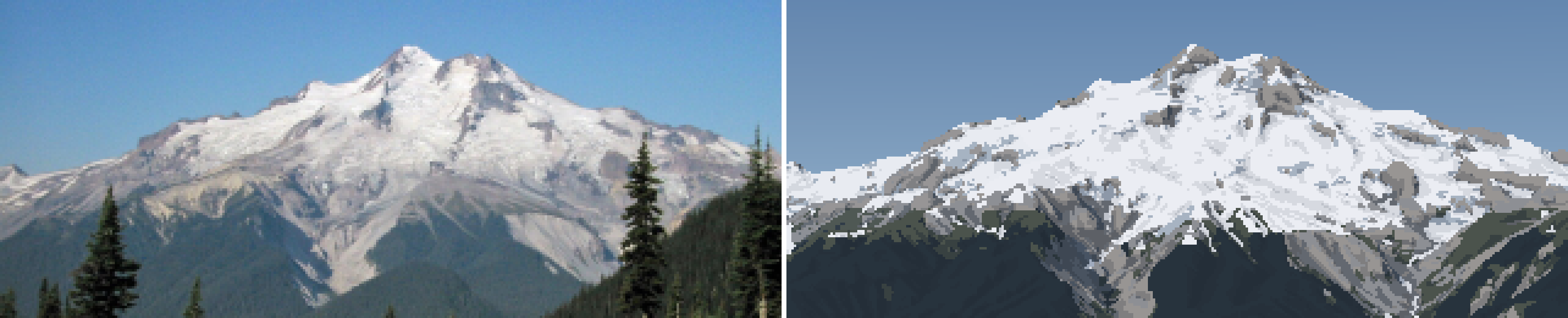
Glacier Peak from the east, 12 km: photo and painting.

Glacier Peak from 12 km, a late-August morning. Left: the photo, box-downsampled to my 320 px grid. Right: my painting of the same view, cast from USGS terrain through the photographer's fitted camera, with the snow placed by a physical model. Shown at 5×.

The one idea

Don't invent the peak. Cast it from the real terrain through the photographer's own camera, then let published snow physics decide where the white goes. Only after that is it painting, and the painting is translation, not invention.

The brief said "match the reference: first its form (the real silhouettes, where the big lights and darks fall, what sits where), then its finer detail." Once the camera is fitted, form stops being an aspiration you approximate by eye. The silhouette is the DEM's silhouette. The big light and dark masses are the real faces under the real sun at the photo's timestamp. The snow sits where gravity, sun and wind would leave it on that exact terrain. And the photo becomes an instrument: every pixel has a known distance and material, so you can measure what haze does at 20 km, or what L* lit snow really has.

real terrain (USGS DEM, lidar, WorldCover ice)
  -> camera fitted to the photo's skyline          how-to 1
  -> snow model: gravity, couloirs, wind, melt      how-to 2
  -> G-buffer per pixel: normal, distance, height, snow, sun
  -> measure the photo through it                   how-to 3
  -> index canvas: material, family, step, haze band -> palette = light     how-to 4
  -> sheets: any distance, season, hour              how-to 5

What I found (numbers a simulation can use)

what	number	where from
snow holding depth on a slope	SHD = 145 m · exp(−0.14 · slope°), min 0.05 m: 2.2 m at 30°, 0.27 m at 45°, 0.03 m at 60°	OGGM Snowslide defaults; chosen over Bernhardt & Schulz by Rainier's bare summer walls
couloirs hold more than open slopes	holding depth × (1 + 3 · gully), gully = concavity at 25 m radius ÷ 4 m	my fit to Stuart: every summer white line is a gully
seasonal snowline, flat undisturbed snow (Cascades)	late May ~1,250 m; early July ~1,900–2,100 m; September minimum ~2,150 m	calibrated on the dated photos (IoU 0.68–0.72 on Rainier)
melt	half air temperature (aspect-blind), half clear-sky insolation with cast shadows	pure-sun melt left white cones in shaded valleys all August
glaciers	WorldCover class 70 is the map. Below 35° the ice keeps its firn; faces steeper than 42° inside the mask are rock	Willis Wall; Glacier Peak's white-over-grey split
lit snow against sky, Rainier at 94 km, clear	+7 L* (65 vs 58), and warmer (b* +11 vs −2)	fitted Seattle photo
the darkest band on a far horizon	the forested foothills: −12 L* under the sky	same
haze depends on height	haze path = distance × mean exp(−h / 2 km) along the ray: forest 5 km below a 2,129 m camera is nearly unhazed	two fitted Rainier photos that one haze distance can't fit
Rainier at dusk, 96 km	snow = sky (73 vs 74): the peak nearly vanishes	fitted Elliott Bay photo
earth curvature	terrain drops d²/(2 R_eff), R_eff = R/0.87: 630 m at 96 km	geometry; visible in every far fit

The how-tos, in reading order

Fit the photo's camera on real terrain. A curved-earth ray caster over the DEM, a panorama cast once from the photo's GPS position, an edge score that survives haze, and the summit control point that made it reliable. Two fits that failed, and why. This is what gets the silhouette and the masses right, and it works for any real place.
Where the snow lies. The snow model as a stack of published rules, each correction forced by a photo: holding depth, couloirs, lidar pits, firn on glaciers, temperature melt. And the instrument that forced them: the model's cover rendered under the photo.
The photo as an instrument. L* per material and distance through the fitted camera, dbg_matL (the photo's values under your own masks), and the altitude-weighted haze path, the single most useful thing I found.
Painting it. Snow decided after fall-line smoothing; lit or shade from the sub-pixel shadow fraction; steps keyed by rank so a face reads at high noon; haze in fine bands of haze path; the palette as light. Taught from the Rainier v1→v16 and Stuart g1→g6 runs, dead ends included.
Sheets, vocabulary, and what isn't there yet. Choosing a standpoint that makes a view, distance × season × light sheets for four peaks, the close vocabulary, and the critics' list.

Where it falls short (read this before copying)

The form half is at the bar: the silhouettes and masses are right by construction, and the snow is in the right places. The surface half isn't:

the rock is a value texture, without the structural strokes Imhof and Ruskin draw;
the terrain under the snow has no ridge-plane structure (a slab at Glacier Peak, camouflage at Stuart 20 km);
lit snow is cold where the photos are warm white;
the close vocabulary (gullies, ledges at 1 m/px) is the weakest part.

Each how-to ends by saying what didn't work.

Running the code

cd ~/work/pixelart-studies/elements/snowpeak/src
export GDAL_DISABLE_READDIR_ON_OPEN=EMPTY_DIR NUMBA_NUM_THREADS=4 OPENBLAS_NUM_THREADS=1
nice -n 10 python3 fitcam.py gp_e_aug                     # fit a photo's camera -> cache/cams.json, stages/fit_gp_e_aug.png
nice -n 10 python3 render.py gp_e_aug sept 320 2100 _x    # photo | painting -> stages/r_gp_e_aug_sept_x.png (+ _crop)
nice -n 10 python3 dbg_matL.py gp_e_aug sept 2100         # photo L* under each painted material vs mine
nice -n 10 python3 sheets.py stuart                       # sheets/A_stuart_distance_season_light.png
nice -n 10 python3 vocab.py                               # sheets/B_vocabulary_scale_season.png

DEM and lidar tiles are read over HTTP from USGS's cloud-optimized GeoTIFFs and cached as small npz boxes in cache/. A 320 px pair at 3× supersampling takes 1–3 minutes and peaks at 1.2 GB RSS, or 2.5 GB with 4 m lidar.