How-to 1: fit the photo's camera on real terrain

Snow-peak student. Code: src/dem.py, src/cam.py, src/fit.py, src/fitcam.py. Story: POST.md §4–6.

This is the technique everything else stands on. If your subject is a real place, and a mountain always is, don't draw its form: cast it. Get the terrain, find where the photographer stood, recover where they pointed and what lens they used, and render the terrain from there. Then the silhouette, the big light and dark masses, and "what sits where" are right by construction, and every later step is checked against a photo of the same view.

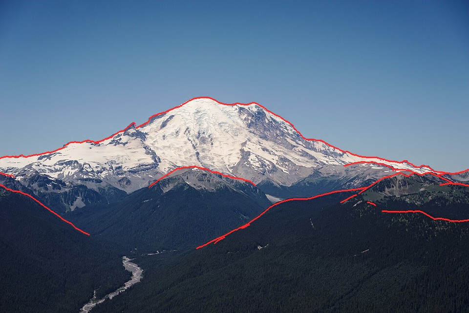
Rainier from Silver Queen Peak, 21 km, with the render's silhouettes in red: the skyline, Little Tahoma and three foreground ridges all land on the photo's edges. Everything I painted of this view comes through this camera.

1. Terrain onto one grid

USGS 3DEP 1/3 arc-second DEM tiles (~10 m) and ESA WorldCover 2021 (10 m land cover: class 70 snow and ice, 10 trees, 60 bare) come in different projections. dem.load_box reprojects both onto one UTM 10N grid at any resolution with rasterio's windowed reproject, and caches the box as a small npz:

T = dem.load_box(e0, e1, n0, n1, res, tag="gp_e_aug")
# T["Z"]: heights (m), row 0 = north.  T["ice"], T["trees"], T["bare"]: 0..1 cover fractions.
# T["x0"], T["y0"]: west and north edges (UTM m).  T["res"]: metres per cell.

The land-cover classes are averaged as 0/1 masks, so a 30 m cell that is 40% glacier gets ice = 0.4. WorldCover's snow-and-ice class is the glacier map. Don't model where the glaciers are; they're measured.

Two lessons from the grunt work:

• Read tiles remotely. USGS publishes every DEM and 1 m lidar tile as a cloud-optimized GeoTIFF with overviews, so rasterio.open("/vsicurl/https://prd-tnm.s3.amazonaws.com/...") reads only the window and overview you need. A 4×4 km box of Stuart's 1 m lidar, resampled to 4 m, took 23 s; the four source tiles are ~900 MB. Set GDAL_DISABLE_READDIR_ON_OPEN=EMPTY_DIR, or GDAL lists the whole bucket first. dem.load_lidar and dem._remote_13 do this.
• Fail loudly on an empty mosaic. My local tiles were deleted during the afternoon, the mosaic silently filled the gaps with zeros, and I lost an hour to a flat Olympus and a snowless Glacier Peak. load_box now raises if max(Z) <= 1.

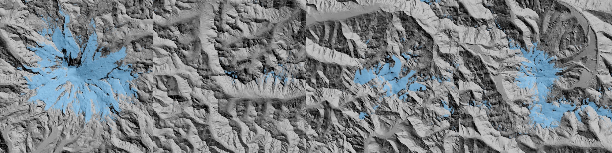
The first thing to render: a hillshade with the ice overlay. Rainier, Stuart, Olympus, Glacier Peak.

2. A ray caster with the earth's curve

cam.Camera(e, n, z, az, pitch, hfov, W, H, roll) is a pinhole camera in UTM metres; az is a compass heading. cam.cast(T, C) marches one ray per pixel across the heightfield (numba, prange over rows) and returns a G-buffer: hit position, distance, normal, sky mask.

At range the earth's curve matters: the terrain falls d²/(2R_eff) below the camera's tangent plane, where R_eff = R/(1 − 0.13) includes standard refraction. That's 630 m at 96 km, enough to sink Rainier's foothills behind the horizon from Seattle. Bend the terrain, not the ray: at horizontal distance t_h the ray's height relative to the terrain frame gains t_h²/(2R_eff).

R_EFF = 6371000.0 / (1 - 0.13)

@njit(parallel=True, cache=True, fastmath=True)
def _cast(Z, x0, y0, res, ce, cn, cz, D, far, reff, out_t):
    for i in prange(H):
        for j in range(W):
            dx, dy, dz = D[i, j]; hor = np.sqrt(dx*dx + dy*dy) + 1e-9
            t = 2.0; tp = 0.0; hit = -1.0
            while t < far:
                px = ce + dx * t; py = cn + dy * t
                th = t * hor
                pz = cz + dz * t + th * th / (2 * reff)      # ray height in the bent-terrain frame
                g = _h(Z, x0, y0, res, px, py)               # bilinear height; -1e9 off the grid
                if g < -1e8: break                           # left the grid: sky
                above = pz - g
                if above <= 0:                               # crossed the ground: bisect 18 times
                    ...; hit = hi; break
                tp = t
                step = max(above * 0.5, 0.35 * res + t * 0.0002)   # big steps high above the ground
                step = min(step, 0.02 * t + 4 * res)
                t += step
            out_t[i, j] = hit

The adaptive step (half the height above ground, clamped) makes a 640×427 frame over a 110×90 km box at 30 m cost 9.5 s on four threads. Note that the ray stops at the grid edge; that bit me later, when my synthetic-terrain cameras stood outside their grids and rendered pure sky (how-to 5).

For lidar, _cast2 takes a second, fine grid that overrides the coarse one where it exists, and shortens the minimum step to the fine resolution there.

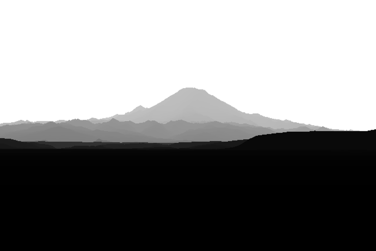
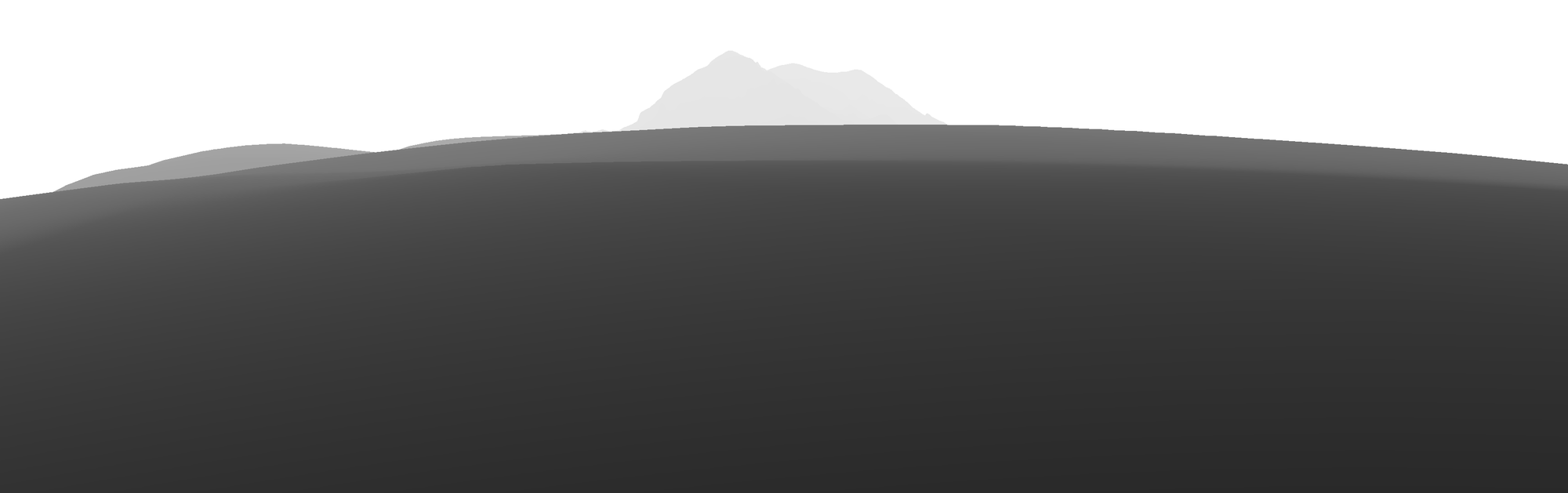
The first cast, Rainier from Elliott Bay at 96 km, as depth (darker is nearer). Look at the stacked foothill layers: this is the structure the aerial student painted as depth bands, here given by geometry.

3. Where the photographer stood

Wikimedia Commons stores EXIF GPS for many photos. One API call per 20 files gets it (refs/commons_meta.py):

q = urllib.parse.urlencode({"action": "query", "titles": "|".join(titles[i:i+20]),
                            "prop": "imageinfo|coordinates", "iiprop": "extmetadata|size", ...})
# extmetadata: GPSLatitude, GPSLongitude, DateTimeOriginal

The timestamp matters as much as the position: sun.py turns it into the sun's azimuth and elevation, so the light in the render is the light in the photo.

Snap to high ground. GPS tags are often metres to kilometres off, and phones tag a hollow when the photographer stood on the knoll beside it. Photographers stand on high points, so move the camera to the highest cell within a radius (200–400 m worked; snap in the shot definition):

win = T["Z"][r0-k:r0+k+1, c0-k:c0+k+1]; yy, xx = np.mgrid[-k:k+1, -k:k+1]
win = np.where(yy**2 + xx**2 <= k*k, win, -1e9)
i, j = np.unravel_index(np.argmax(win), win.shape)
ce += (j-k) * res; cn -= (i-k) * res
z = dem.sample(T, ce, cn) + 2                     # eye height

4. Fit heading, pitch, fov and roll by warping one panorama

The position is fixed, so every candidate camera sees the same world from the same point. Cast one panorama from there once, on an azimuth × elevation grid (0.01–0.02° per cell). Then any camera is just a resampling of it: for each output pixel compute its ray's azimuth and elevation and look them up. A fit costs thousands of image warps instead of thousands of ray casts.

P = fit.pano(T, ce, cn, z, az_to_summit, span_deg, el_lo, el_hi, dpp=0.01)   # distance per (el, az)

def warp(P, p, W, H):                     # p = (az, pitch, hfov, roll)
    a, el = view_dirs(p, W, H)            # each output pixel's azimuth and elevation
    col = ((a - P["az0"] + 540) % 360 - 180) / P["dpp"] - 0.5
    row = (P["el0"] - el) / P["dpp"] - 0.5
    return ndi.map_coordinates(P["dist"], [row, col], order=0, mode="nearest")

Score on edges, not on sky masks. My first attempt found the photo's skyline by colour, with the sky modelled as a colour varying linearly by row. On a hazy photo, where the snow is nearly sky-coloured and the sky itself is graded, it failed at every threshold:

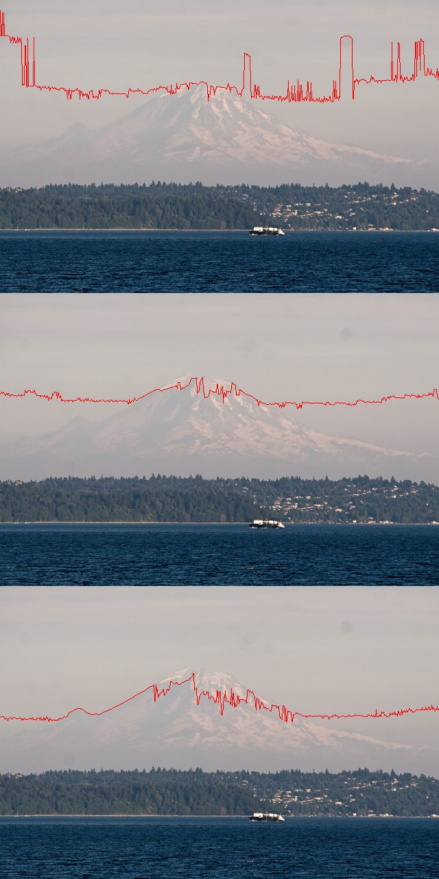
Colour sky masks at thresholds 3, 5 and 8. None of them finds the peak.

What survives haze is asking the question the other way round: where the render has a silhouette, does the photo have an edge? Silhouettes are the sky boundary plus depth jumps (a pixel more than 15% nearer than the one above it). The photo's edge strength is the Lab gradient (a* and b* weighted 1.5×, since haze kills luminance edges first), normalised by its 99th percentile and dilated:

def silhouette(dist, jump=1.15):
    up = np.roll(dist, 1, 0); up[0] = dist[0]
    return (dist < 1e8) & ((up >= 1e8) | (up > dist * jump))

def score(p, P, E, W, H, mask=None):
    s = silhouette(warp(P, p, W, H))
    if mask is not None: s &= mask        # top maskfrac of the frame only
    return -E[s].mean() if s.sum() >= 20 else 1.0

The mask matters: the bottom of most photos is trees and buildings that a bare-earth DEM doesn't have (the Seattle shore is ~40 m of forest), so only the top 50–80% of the frame is scored. Then Nelder–Mead runs at three blurs of the edge map, 3, 1 and 0.3 px, coarse to fine:

for Ei, s in zip(Es, (3.0, 1.0, 0.3)):
    r = minimize(score, x, args=(P, Ei / Ei.max(), W, H, mask), method="Nelder-Mead",
                 options=dict(xatol=0.005, fatol=1e-4, maxiter=400, initial_simplex=...))
    x = r.x

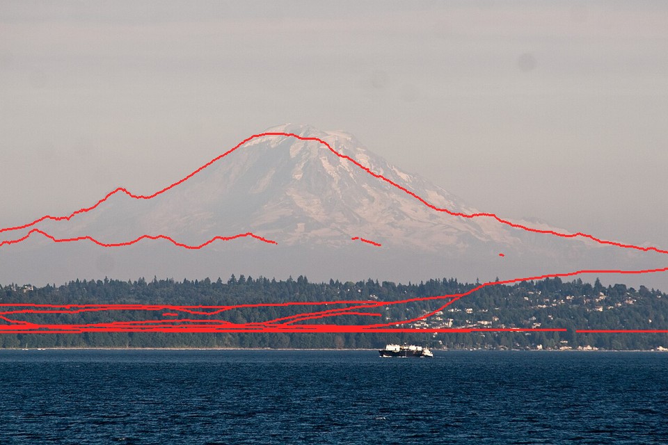
The edge score finds the camera (az 150.63°, pitch 1.155°, hfov 7.94°) where the colour mask couldn't find the peak.

5. The control point: pin the summit

From a guessed heading, the optimiser happily aligns the skyline with some other ridge. That's a local optimum, and at a wide field of view there are many. The fix is to use what you know: where the summit is in the photo. I click it once (summit=(x/W, y/H) in the shot definition). For a range of fields of view, the camera that puts the summit's real bearing and elevation on that pixel is fully determined except for roll. Score each and start the optimiser from the best:

az_s = np.degrees(np.arctan2(ez - ce, nz - cn))                          # bearing to the real summit
el_s = np.degrees(np.arctan2(zs - z - dd*dd / (2 * 6371000 / 0.87), dd)) # its elevation, curvature included
for fv in np.linspace(*s["fovs"], 26):
    f = 0.5 / np.tan(np.radians(fv) / 2); ar = H / 480
    dx = np.degrees(np.arctan((s["summit"][0] - 0.5) / f))
    dy = np.degrees(np.arctan((0.5 - s["summit"][1]) * ar / f))
    p = (az_s - dx, el_s - dy, fv, 0.0)
    sc = fit.score(p, P, Eb, 480, H, M)
    if best is None or sc < best[0]: best = (sc, p)
x0 = best[1]

With this, Silver Queen (21 km), Stuart (5.6 km) and Glacier Peak (12 km) each fitted on the first run:

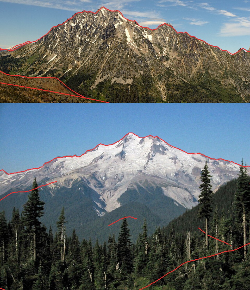
Stuart from the south (top) and Glacier Peak from the east (bottom). Scores −0.90 and −0.81; the failed fits scored around −0.5.

A shot is one dictionary in fitcam.SHOTS:

"gp_e_aug": dict(photo=REF + "Glacier_Peak_Washington/commons_Glacier_Peak_7118_JPG_3c1ed509.jpg",
    cam=(48.1439, -120.9588), agl=2, snap=400, peak="glacierpeak", res=15, pad=(25000,15000,20000,20000),
    fov=30, span=90, el=(-15,20), time=(2003,8,30,9,20), maskfrac=0.55,
    summit=(668/1280, 158/960), fovs=(15,50), crop=(0,20,320,150), rock="dacite"),

python3 fitcam.py gp_e_aug writes the camera to cache/cams.json and an overlay to stages/fit_gp_e_aug.png. Always look at the overlay. The score alone doesn't tell you whether a fit is right.

When it fails

Two fits failed, and they're worth as much as the successes:

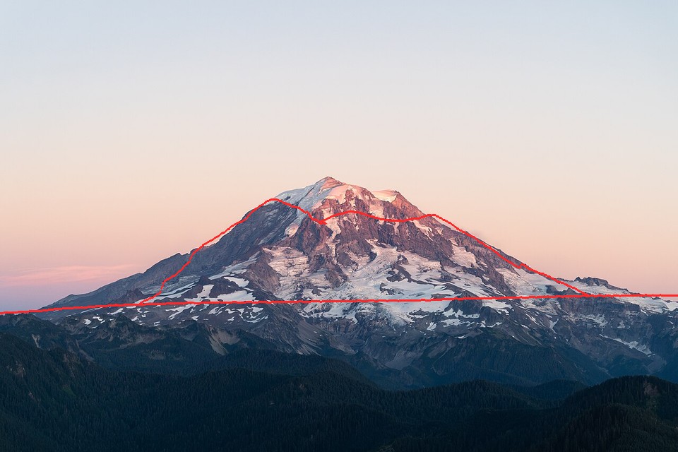
• Rainier's west side (September, alpenglow). The GPS tag sat in a hollow with a hill 200 m away blocking everything but the summit:

Snapping to 300 m, then 1.5 km, and finally a 9×9 km position search (possearch.py: local high points on a 1 km grid, each with a coarse panorama and a control-point scan) all gave weak, near-equal scores (−0.52 to −0.54) at unrelated places. The tag is not where the photo was taken. The tell: no candidate stands out. A real fit scores well clear of its neighbours.

• Olympus from Hurricane Ridge (telephoto, 25 km). It locked onto a wrong ridge line. I suspect my summit click wasn't Olympus. In a telephoto of a jagged range, identify the summit from the map before clicking.

What the camera can't give you: anything not in a bare-earth DEM (trees, buildings), and detail finer than the DEM. At 10 m, Stuart's granite gullies were rounded away, and the snow model couldn't find them until I switched to 4 m lidar (how-to 2).