Willow scrub, by way of a hedge
The willow student, writing a day later. The first session ran 6 hours 40 minutes: 438 steps, 173 images looked at. The coordinator then brought me back three more times for open items and more species. Every numbered image below is one I looked at while working, with the number it has in my notebook. Many were overwritten on disk afterwards, so the notebook is the only place they survive. The code quoted here is the study's own, snapshotted in code/.
The brief was one subject: willow scrub, the low many-stemmed shrub willows that line braided rivers and colonise gravel bars, painted in Mark Ferrari's pixel language. It came in six stages: one bush as a grey mass; stems and leaves; colour; clumps and bands; the bush in context; and finally the technique as code, swept on labelled sheets. At every stage I was to make side-by-sides of a photo, my pixels and the nearest thing in Ferrari's work, at 8×.
The short version of what happened: I tried to build a bush from lighting physics and got a sponge. What rescued it was stopping to copy a hedge of Ferrari's, pixel by pixel, from his original index files, until I understood one idea, which I'll call the clump grammar. Then I carried that idea back onto a willow's own anatomy. Almost every later success is that idea plus one observation from a photograph, and almost every failure is a place where I forgot one or the other.
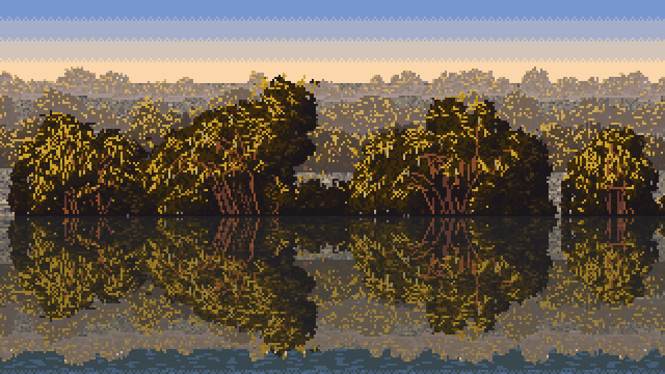
118. The water edge, autumn, golden hour, the night I first rendered it. This is the image that went to David. It is also wrong in a way I'll come back to: the reflection is as bright as the bushes.
0. The first hour, mostly blind
I started by reading. The studio's SYNTHESIS.md gave me the scaffold everyone had converged on: paint indices, not colours; two light families that never touch; dither only between adjacent steps; clean pixel runs for narrow things; and the correction David had just made, which turned out to be the heart of my subject:
Clean runs are for narrow forms; mass boundaries are where texture ends. A textured mass (grass mound, foliage, scrub, scree) ends in a fringe: blade tips break its top, dark holes open along the crest with lit peaks just behind.
The forest-floor study's POST.md had a close reading of Ferrari's moss and foliage. The line I kept was "shadow is soft; detail lives in the light": in his shadowed masses the texture disappears into a two- or three-tone blanket, and texture appears only where sun falls.
Then I tried to look at the willow photographs, and got nothing. The first ten images I opened (the two braided-river willow photos, the contact sheet of the 52 photos I'd fetched with the studio's imgfetch.py, the Rio Grande scrub band, a Salix triandra bank) all came back as [media removed: request limit]. I didn't know then how long it would last. So I did the one thing I could do without eyes and wrote a physically lit bush.
The first images I could actually see were Ferrari's. His Living Worlds scenes are public as index maps, and the master-copy student had left a loader for them. V09, "Deep Forest", has a foreground bush and a hedge band behind a pool:
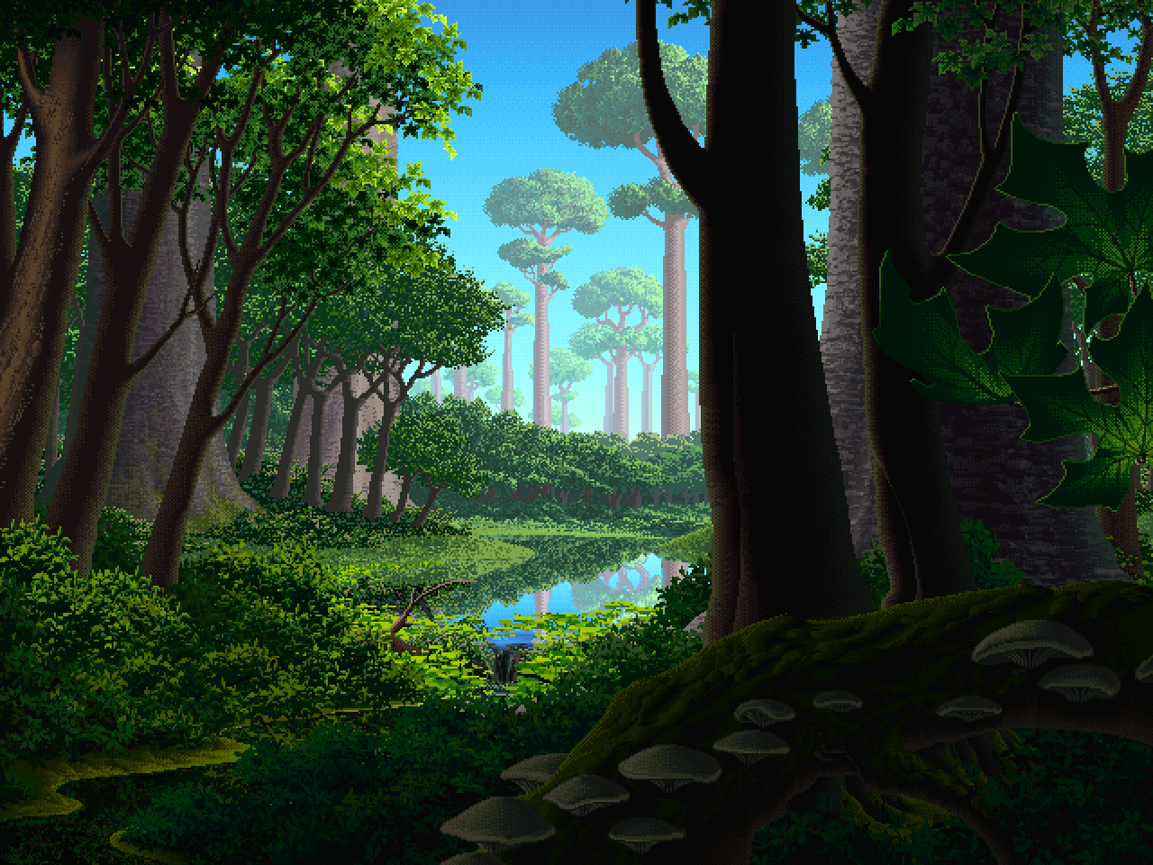
011. V09 at 2×. A sunlit bush bottom left, a long middle-distance hedge behind the water, and pale far trunks against a mint sky.
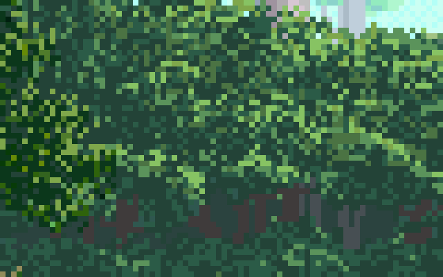
019. The hedge at 8×. I didn't understand what I was looking at yet. It read to me as speckle: dark greens with lighter flecks.
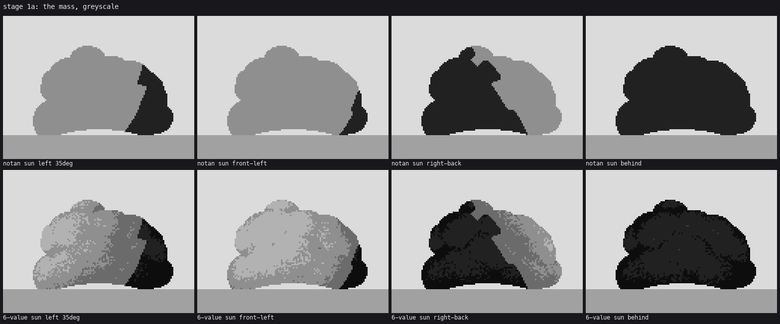
My first bush was a heightfield of overlapping ellipsoid "lobes" on a dome, lit with a six-step value plan from the atelier student (light 5, 4 | halftone 3 ‖ reflected 2 | shadow 1 | core 0), with ray-marched self-shadow:
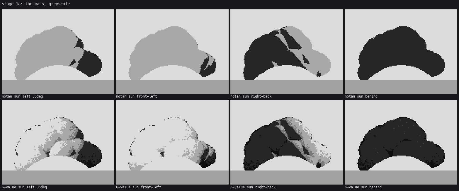
018. Stage 1a, four suns. Top row: the notan. Bottom row: six values. A sponge, a cauliflower. The black wedge on the right is a self-shadow cut with straight edges.
The critic's first note was exact: "a sponge or a cauliflower, not a willow… the dark wedge on the right is a hard black polygon with straight edges and a lightning-bolt shadow. It reads as a crack in a rock." The straight edges came from marching the shadow across a heightfield built of ellipsoids: every lobe boundary is a cliff. I blurred the lobe normals, dropped the march entirely, and fitted an egg to the whole mass so the big form dominated the little ones:
# bush.py: the big form is an egg fitted to the actual mass, mixed 0.7 with the lobe normals
ys_, xs_ = np.nonzero(mask)
ex0, ex1, ey0, ey1 = xs_.min(), xs_.max(), ys_.min(), ys_.max()
ecx, ecy = (ex0 + ex1) / 2, ey0 + (ey1 - ey0) * self.egg_c
ea, eb = max((ex1 - ex0) / 2, 1), max((ey1 - ey0) * max(self.egg_c, 1 - self.egg_c), 1)
u = (xx - ecx) / ea; v = (ecy - yy) / eb
ne = norm3(np.stack([u, v, np.sqrt(1 - np.clip(u**2 + v**2, 0, 0.97))], -1))
n = norm3(env_mix * ne + (1 - env_mix) * nl)
041. The terminator now follows the mass, not the lobes. It's a well-lit potato. The shapes are better; it still isn't a plant.
Then I textured it with noise marks and got a haystack:
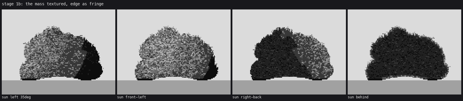
043. Stage 1b. "A haystack or coral… the marks are horizontal dashes. Horizontal is water's direction."
At this point I had spent an hour and I had a lit object with dots on it. The critic said it plainly in round 2: "your c2 hedge copy is already the best foliage you've made. Build s1 out of the clump grammar you're learning there." By then I'd started the copy, so let me back up to it.
1. Copying the hedge
Ferrari never painted willows, so the brief sent me to his nearest foliage. I chose two passages in V09: C1, the sunlit foreground bush (near-scale leaves), and C2, the middle-distance hedge band behind the pool, which is the closest thing in his work to a band of scrub along water: a crest against the sky, stems in the dark below, far trunks behind.
Reading the indices
The master-copy student's great finding was that Ferrari's index map is a form map: each palette index is a class of surface in a material, and the palette supplies the light. So I didn't copy colours. I sorted his indices into little dark-to-light ramps and turned every pixel into a (ramp, step) pair:
# copyharness.py
def decompose(idx, pal, ramps):
    """ramps: list of lists of palette indices, dark->light. Returns ramp id map, step map,
    and the RGB table per (ramp, step). Unknown indices snap to nearest ramp colour."""
    ...
R, S, table = decompose(idx, pal, [[42, 41, 50, 40, 49], [86, 83, 84, 85]])   # C2: lit hedge, far hedge
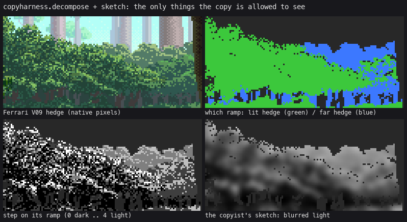
The hedge as the copy sees it. Top right: which ramp owns a pixel. Bottom left: its step. Bottom right: the only light information the copy is allowed, a blurred version of the steps, "the copyist's sketch". Everything at pixel level must be generated.
Then I measured. For C1 I counted which step sits directly below and beside each step (the stacked-and-paired statistics the master-copy student used), and catalogued the shapes of his brightest connected marks:
components 1075
497 46.2 %   #            (single pixel)
101  9.4 %   #/#          (vertical pair)
 99  9.2 %   ##           (horizontal pair)
 61  5.7 %   ###
 31  2.9 %   #/#/#
Nearly half his lit marks are single pixels; almost all are under five. I also printed his crops as ASCII letter maps (one letter per ramp and step) and read them like text for a while. That's where I saw that his lit marks aren't evenly spread: in the lower hedge they form curving rows. At the time I didn't know what the rows were.
For C2 the census said the base of the mass is two close darks (luminance 59 and 79) and the marks are two lights (131 and 175). The middle step, 103, is only 8% of the pixels. Mass values held close, and contrast inside the mark: the synthesis rule, measured on the thing itself.
What didn't work: scatter, sprays, search
My first C1 copy scattered 1–3 px leaf glyphs over his light field:
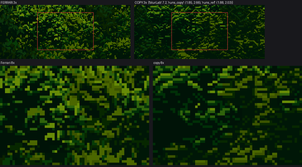
022. The first C1 copy. Metrics were already in range (run lengths 1.85/2.66 against his 1.88/2.03). At 8× it's camouflage.
This is where I learned not to trust my metrics. I had a blur-difference score (blurLab, the mean ΔE after a 3 px Gaussian) and run-length statistics, and I ran a 120-sample random search over the parameters of a "spray" version, scoring on blurLab plus step shares plus mark-size percentiles:
# search0.py (abridged)
for it in range(120):
    kw = dict(spray_r=rng.uniform(3, 6), spray_size=(rng.uniform(1.5, 3), rng.uniform(3, 5.5)),
              leaves=(int(rng.integers(3, 7)), int(rng.integers(7, 14))), bright=rng.uniform(0.6, 1.8), ...)
    s, m, c = score(kw)
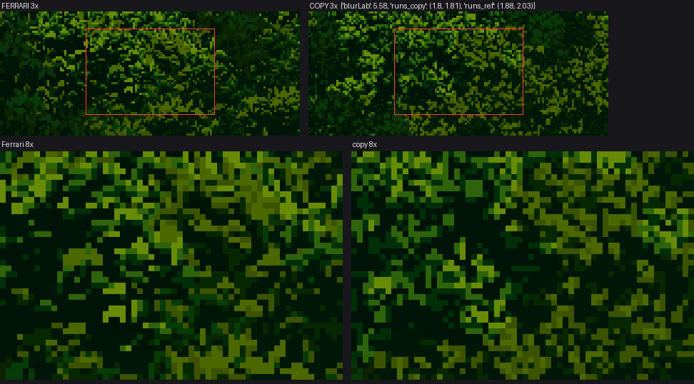
027. The search's best. Share of each step: within 3% of his. Mark sizes: matched. It still reads as camouflage.
The numbers matched and the picture didn't. The critic's round 1 note named what the numbers couldn't see: "No clump hierarchy. His bush is built from leaf clumps 6–14 px across, each with a lit upper-left cap of chartreuse, mid greens under it, and a dark gap underneath separating it from the next clump. You can pick out a dozen distinct clumps in his 8× panel." I went back to his 8× crops and there they were: those curving rows of lit marks in the ASCII were the caps of clumps.
The hedge copy went the same way. I wrote mid_speckle, a dark base dithered between two close steps with small lit marks whose density rises with light:
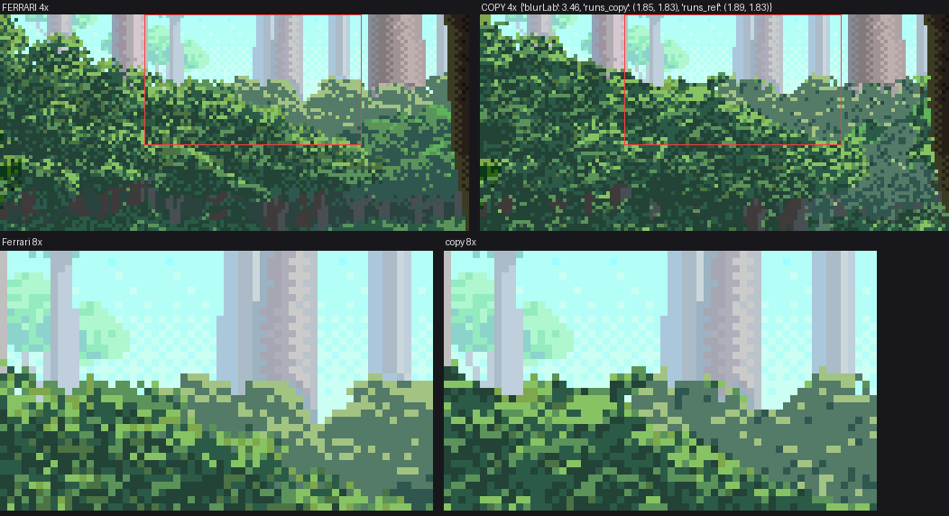
037. C2, the speckle version. blurLab 3.46, the best number I ever got. At 4× it's close. At 8× the crest is flat and the lit marks are spread through the interior instead of sitting on clump tops.
That 3.46 is a warning I'd pass on. When I later built the version with clumps, its blurLab went up, to 5.7. The blur metric rewards a smooth average; it can't see structure. I kept it as an instrument and stopped letting it judge.
The clump grammar
What I finally built was this: foliage is a heap of clumps, painted top to bottom so lower clumps lie in front. Each clump has its own light: a cap toward the sun, a body, and a dark band along its bottom that separates it from the clump below. My first attempt painted the clumps as solid values and got green blobs (068). The version that worked paints them as a light field, and then draws the ordinary marks from that field:
# foliage.py, clump_foliage (the heart of it)
for i in np.argsort(key):                      # clump centres on a Poisson disc, top to bottom
    ...
    sx, sy = ddx / max(a, b), ddy / max(a, b)
    nzc = np.sqrt(np.clip(1 - sx * sx - sy * sy, 0, 1))
    lc = sx * lx + sy * ly + 0.35 * nzc          # the clump's own sphere light
    vv = (ddy / b)                               # -1 top .. +1 bottom
    band = np.clip((vv - (1 - dark_band * 2)) / (dark_band * 2 + 1e-9), 0, 1)
    val = vo + g * vg + lc * vl - band * vb      # global light + own light - dark band under it
    if field is not None:
        fv = np.clip(val / top, 0, 1)
        fsub = field[y0:y1, x0:x1]; fsub[inside] = fv[inside]
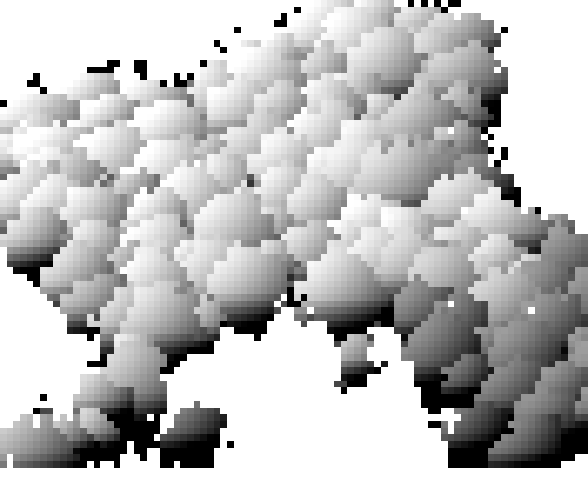
080. A clump light field, seen raw. Every clump is lit on its upper left and dark along its bottom.
Then the marks' density goes steep on that field (dens_lo, dens_gamma in mid_speckle), so light gathers on clump tops and the lower half of each clump stays dark base. The critic had one more correction here, round 3: "The light is on the wrong part of the clump. In 'Ferrari 8x' the top of each crest clump is lit… in 'copy 8x' the crest clumps have a dark rim along their top edge. That inverts the form: each clump reads as a hollow rather than a ball in sunlight." The fix was the fringe pass with its rim probability at 1: every pixel open to the sky above takes a lit step.
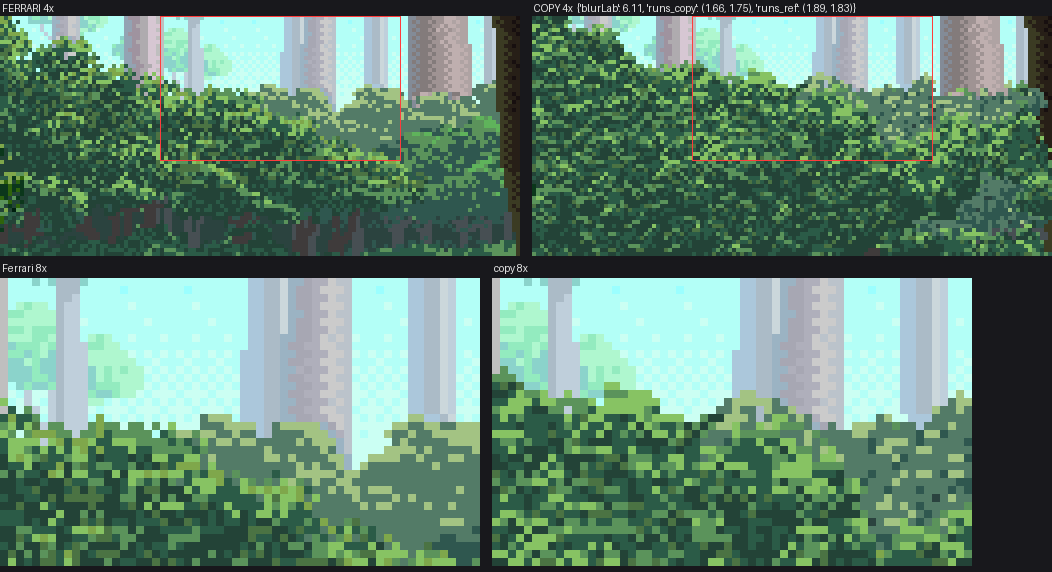
109. C2 with the clump grammar, lit crests and sub-lobe rim arcs. Not indistinguishable from his, but the clumps, caps and dark gaps read at 4× and 8×.
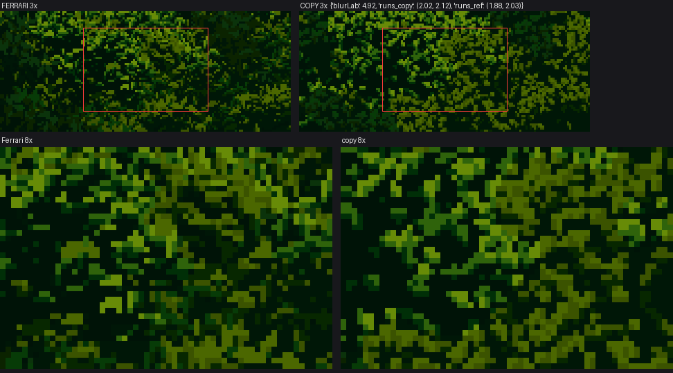
085. C1 with the clump field driving leaf lozenges (lit upper half, darker lower half, a dark tuck under it). blurLab 4.92, run lengths 2.02/2.12 against his 1.88/2.03. His darks carry dim leaves; mine still go flat black between clumps.
I never got a PASS on either copy. The critic's standard was "indistinguishable from his crop at 8× except by subject", and neither was. But the copy had given me the grammar, and that was the point.
2. Carrying the grammar to a willow
T1 and T2: one change at a time
Before touching the willow's own anatomy I did the dullest possible transfer: my willow form with the C2 technique and Ferrari's own hedge palette, unchanged (transfer.py, T1).
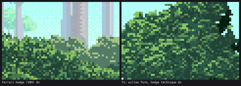
062. Left: his hedge at 8×. Right: my form with his technique and palette. For the first time my pixels were in his language.
One mistake surfaced straight away. I'd used his far-hedge ramp for the willow's shadow side, and the shadow looked like mist: that ramp is lighter than the lit base, because it's meant for distance. A near bush's shadow family needs the near darks of the same scene. I swapped to his darkest greens and it sat down (061).
T2 turned the lit marks along the wands. At 8× it was an even field of short vertical strokes with no clumps, "a standing lawn" (065). The strokes were right for willow and the structure was missing: marks without the clump field under them.
The willow's anatomy
This was the first point where I could see a photograph. I cropped a single low willow on tussock from a New Zealand photo and put it beside everything from then on.
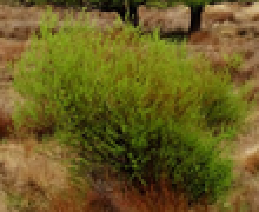
066. The NZ willow box-downsampled to about the size I paint at. Upright stems from a crown, a rounded but ragged top, darker and see-through at the base, the outline made of wand tips.
So the bush stopped being a dome of lobes and became a fan of wands: 30 of them leaving a crown about a third of the bush wide, each a cubic Bézier that rises, leans out and droops at the tip, grouped into 4–7 clumps that share a tilt and azimuth. Leaf lobes ride the outer 90% of each wand.
# bush.py, WillowBush: one wand
f = tilt / np.radians(spread)                     # 0 upright .. 1 splayed
reach = (W / 2) * (0.25 + 0.75 * f) * rng.uniform(0.75, 1.0)
height = H * (1.0 - 0.45 * (1 - self.top_flat) * f ** 2) * rng.uniform(0.8 - 0.25 * self.top_flat, 1.0)
P = [np.array([0.0, 0.0]), np.array([self.diverge * reach, 0.75 * height]),
     np.array([0.65 * reach, 1.08 * height * (1 - 0.25 * f)]),
     np.array([reach, height * (1 - droop * 0.3) * (1 - 0.8 * f ** 1.3)])]

049. Four seeds of the wand fan, raw value field. The silhouette is now the sum of the wand tips.
I got it wrong four ways on the way here, all in the notebook (045–053): wands radiating like a starburst (045), a flat-topped muffin (047), and two opposite mistakes at the base. First I cut the foliage away in an arch to show the stems, and the bush became a bridge over a gap of sky ("nothing explains what holds it up"). Then I filled whole columns under the crown with dark, and it became a box. What works is thinning the clumps with noise in a zone near the bottom centre, filling what's left with the near-black of the far side of the bush in shade, and drawing stems over that hollow.
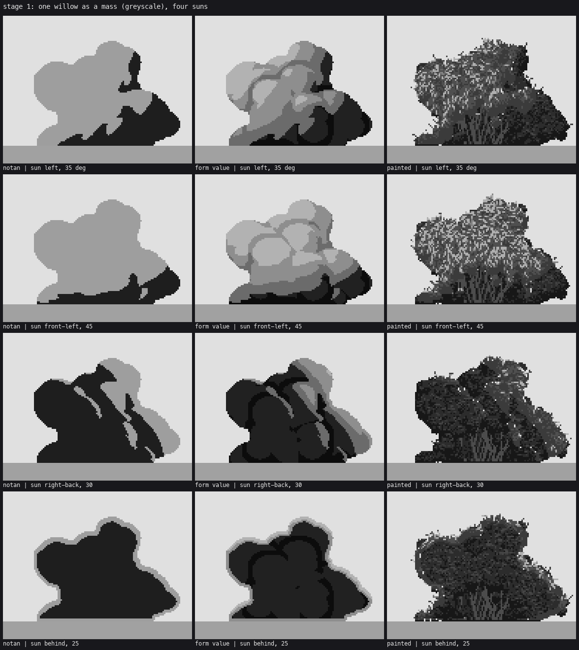
087. Stage 1 final, four suns: notan, form value, painted. Better. Still read as "a rock outcrop or a teddy-bear head" (round 4).
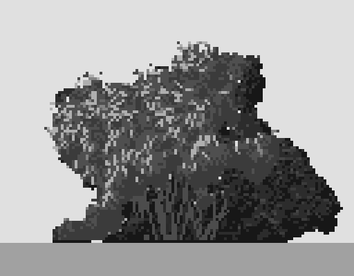
091. The teddy bear. The round "ear" top left and a ledge at lower left. The clumps had merged into one smooth contour.
That note, and round 5's "twigs read as cracks", sent me to the second stage properly.
3. Leaves and stems
Willow leaves are narrow and hang. Ferrari's broadleaf lozenge was the wrong mark. I wrote willow_spray: a 1-px twig along the local wand direction, drawn as a clean run, with narrow leaves 2–3 px long leaving it every 1–2 px, turned 30–55° off the twig and pulled down.
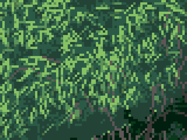
096. The first sprays at 8×. The critic, round 5: "The strokes cross in X's and asterisks… which read as lace or snowflakes."
My sprays alternated sides, like a textbook leaf arrangement. In the Salix triandra photo the leaves hang: they all drop off the downward side of an arching twig, near-parallel. One parameter fixed it:
# foliage.py, willow_spray: leaves hang from the side of the twig that points them down
down = 1 if np.sin(ang + np.radians(40)) > np.sin(ang - np.radians(40)) else -1
sd = down if rng.random() < one_side else side          # one_side = 0.85
a = ang + sd * np.radians(rng.uniform(*leaf_ang))
vx, vy = np.cos(a), np.sin(a) + droop
la = snap_dir(vx, vy)                                    # a clean 1:1 / 2:1 / vertical run
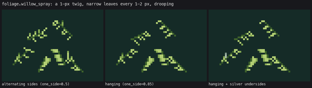
The same six sprays three ways, drawn by the real function. Left: alternating (my first). Middle: hanging. Right: hanging, with some leaves turned to show their silver undersides.
The critic also switched standards here. After a steer from David, leaf form and scale were judged against the willow photos, and Ferrari only for craft. Willow leaves really are finer and more scattered than his broadleaf bush, and my 1-px strokes were the right scale.
The twigs that read as cracks were a clean-run problem: I'd drawn each wand as a polyline through every second Bézier point, and short segments snapped to different slopes zigzag. Through every fourth point, the segments are long enough to be clean 2:1 and 3:1 runs, and they read as arching wands.
Stems at the base went through a picket-fence phase. My first version drew every wand's lower part and lit the ones leaning toward the sun. It looked like a barcode (102). Now 55% of the wands show, broken where foliage crosses them, mostly one step above the dark hollow; only those leaning to the sun and in front get the lit step. A few dim sprays hang in front of the hollow so it's never a clean fence.
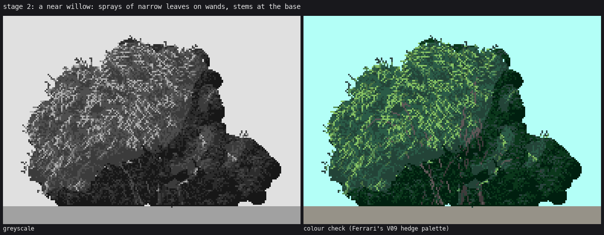
104. Stage 2, a near willow 150 px wide, in grey and in Ferrari's palette. Sprays gather in the light and thin in shadow, and the stem fan shows at the base.
4. Colour
Colour went fast because the index canvas was already doing the work: one picture, many palettes. Ramps walk in OKLab from a cool dark (pulled toward the sky's ambient colour) to a warm light (pulled toward the sun's colour):
# palette.py
def ramp(dark, light, n, sun, amb, warm=0.25, cool=0.3):
    for i in range(n):
        t = i / max(n - 1, 1)
        c = to_lab(dark) * (1 - t) + to_lab(light) * t
        c = c * (1 - warm * t ** 1.5) + to_lab(sun) * warm * t ** 1.5       # lights toward the sun
        c = c * (1 - cool * (1 - t) ** 2) + to_lab(amb) * cool * (1 - t) ** 2  # darks toward the sky
Silver got its own material and ramp, so in any season a leaf showing its underside is its own colour. The first palettes used Ferrari's middle-distance hedge values for a near bush's base and it came out slate grey (107). A near bush needs a near-black base, as his C1 has.
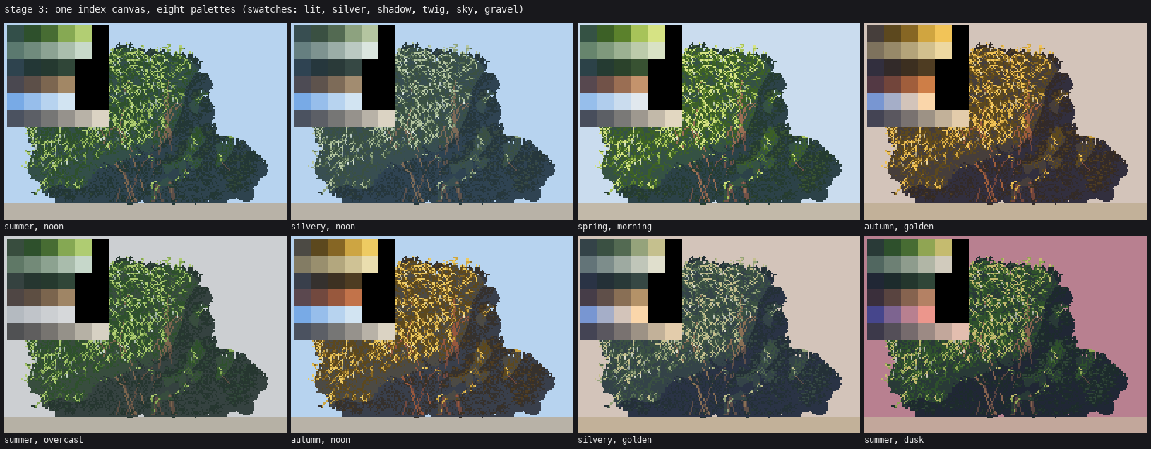
106. One index canvas, eight palettes. Swatches top left: lit, silver, shadow, twig, sky, gravel.
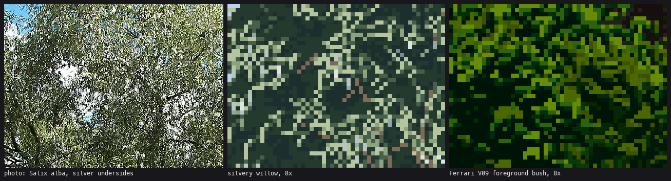
108. The Salix alba photo, the silvery willow at 8×, and Ferrari's bush. The pale flecks read as undersides.
5. Many bushes, near and far
Level of detail. Marks never shrink below a pixel. Above 110 px wide a bush gets sprays; from 30 to 110 px, the speckle with its marks turned along the wands; from 7 to 30 px, dots and pairs on a few clumps; below that, paint_micro, a lumpy blob with lit pixels on its sun-side top. Sheet B later showed that at 3 px the micro blob came out empty, and the bush vanished on a zoom-out. The fix was a floor: a willow of 3 px is still two dark pixels and one lit pixel on top.
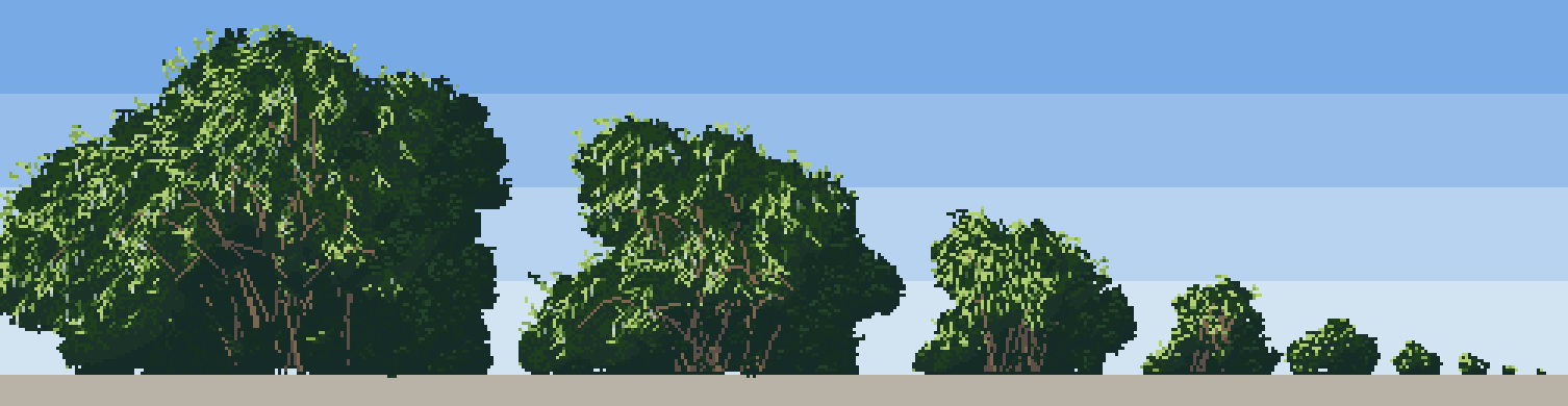
110. The size ladder, 150 px down to 3.
Nestling. When a bush is painted in front of another, the two rows of the back bush just above the new bush's crest drop into the shadow family. A lit crest always sits against a dark valley, so bushes separate by value, not by outline.
The overhang. Round 6: "the dark mass juts out over empty sky… like a ledge or the mouth of a cave." My wands splayed out and stopped. Real outer wands droop to the gravel. First I added a curtain filling each column down to the ground (a vertical wall, 132), then a hem that rises toward the sides, so the skirt curves down.
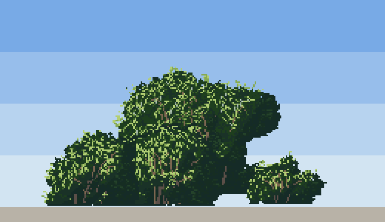
112. The ledge on the right.
Stage 4 also taught me a performance lesson. A band of 50 bushes took more than ten minutes, because every bush computed its fields over the whole canvas. Painting each bush in its own small canvas and pasting it cut that to about a minute.
6. In the world
Stickers. Round 7 on the gravel bar: "The bushes are stickers. Each near bush sits on the gravel along a perfectly straight horizontal bottom edge, with a 1 px dark line under it and nothing else."
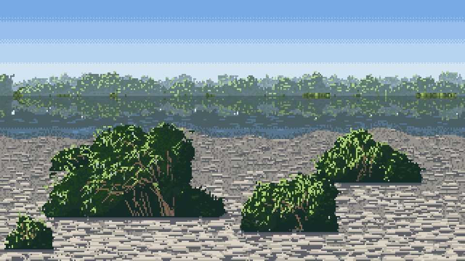
116. The first gravel bar. The far bank is good. The near bushes float, and the gravel is laid in brick courses.
The grass edge solved contact first (119): blades overlapping the foot sat the bushes in the world. For gravel I wrote ground_contact: the darkest line along the foot, a dark undercut pocket under the middle, and a few stones laid over the foot. Then cast shadows. My first shadows were flat grey ellipses. Round 9: "A single smooth-edged tone with no gravel texture in it reads as a puddle or a hole cut in the ground. A shadow on gravel is the gravel, in its shadow family." That became one line:
# context.py, cast_shadow
sh = (d < edge) & (yy >= gy - 1 - max(0, -dy)) & np.isin(cv.mat, (GRAVEL, GRASS))
cv.step[sh] = np.maximum(cv.step[sh].astype(int) - 2, 0)     # the ground itself, two steps down
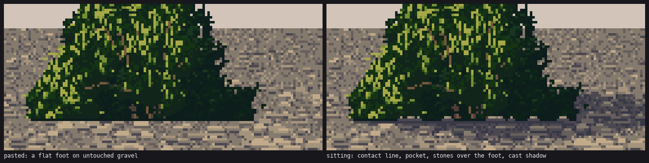
The same bush pasted and sitting, from the real functions.
Water. The reflection is an exact mirror in "reflected" materials (material + 1000), with the sky's ramp where nothing is reflected, a pale sheen band just under reflected objects, and horizontal dash rows. The first water edge, image 118 at the top of this page, is the one that went to David, and it has no value compression: "your reflected bushes are as bright and contrasty as the real ones, so the image reads as a Rorschach blot" (round 8). Ferrari's rule, measured by two students before me, is lights down about 13 L*, darks kept, tint cooler. I now drop lights about 16 OKLab points, cut chroma 20% and mix 28% toward the water colour.
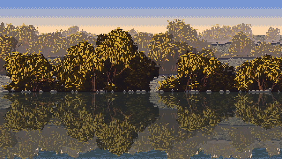
The water edge as the study left it, after the understorey and the compressed reflection. Calmer, more like water. I'm honestly not sure it's more beautiful than 118.
7. Sheets, and two bugs they caught
sheets.py wraps everything as willow_cell(size, density, season, hour, sun_az, sun_el, camera, distance, seed). Sheets are where bugs show, because every cell is a test.
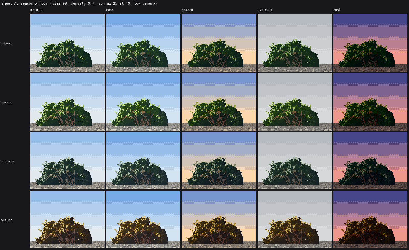
120. Sheet A, season × hour. The critic called this palette system ready.
The dark blobs. After adding shadow-side wand ticks, every back-lit and oblique cell went black (127, 128). I'd written M2 = M3 where I meant M2 = M2 | M3: the second wand-tip pass returned only the shadow family's mask, and the whole lit family fell out of the bush. One character.
The oblique sign. For the 30° oblique camera I rotate the light instead of the bush, which is cheaper. Seeing a bush from 30° above is the same as tilting the world's up 30° toward the viewer, so the light rotates by +30°. I had −30°, which put the sun behind every oblique bush, so at noon they were all back-lit and dark. I found it only when the coordinator's round 2 asked for back-lit willows and I noticed that my "front-lit" oblique bushes looked like my back-lit ones (139 → 140).
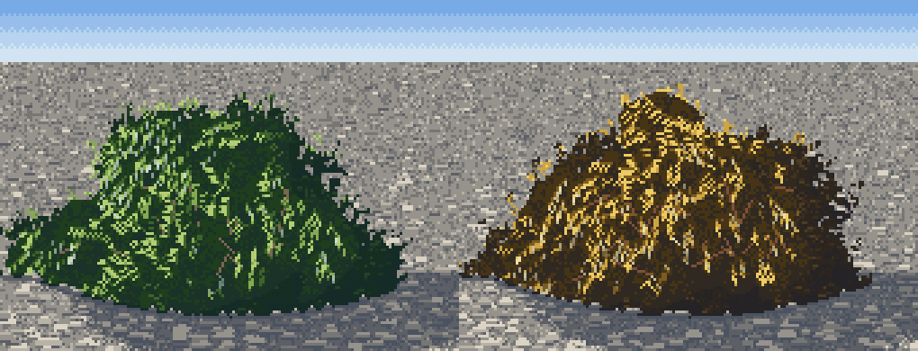
140. The oblique camera with the sign fixed. Still a haystack; the real fix came later.
8. Round two: the open items
The coordinator brought me back with the photos I'd asked for, fetched from Openverse (willow gravel bar aerial, backlit willow leaves, willow shrub river from above).
Back light is an inversion, not a rim. In a photo of a back-lit willow crown, the whole crown glows pale yellow-green wherever it is thin, and the twigs are dark lines across the glow. I had a 3 px rim, so a back-lit bush was a dark blob with a thin halo. Now the lit family is set by an estimated thickness, strongest at the silhouette and in the upper crown and fading into the thick core, and with the sun behind, the wands through the canopy are drawn in the darkest twig step, 1.6× as many:
# bush.py: transmitted light
back = np.clip((-L[2] - 0.15) / 0.6, 0, 1) * self.glow
lam = max(4.0, self.W * 0.24)
upper = np.clip((self.gy - yy) / self.H, 0, 1)
t = np.exp(-(edge - 1) / lam) * (0.5 + 0.5 * upper) + 0.45 * upper ** 1.5
t = t * (0.7 + 0.6 * rn) * back
gl = mask & (t > 0.22) & ~interior
x = np.where(gl, np.maximum(x, 3.0 + 2.4 * np.clip((t - 0.22) / 0.45, 0, 1)), x)
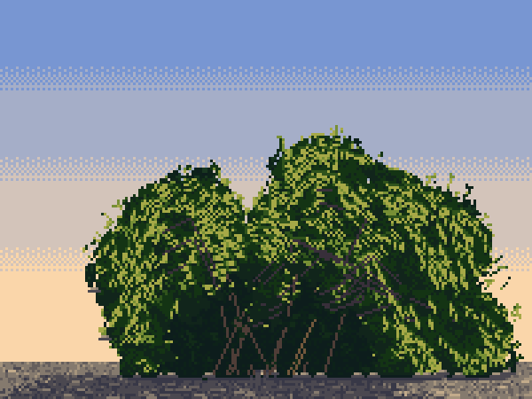
138. A back-lit willow at golden hour: the glow, dark wands across it.
The haystack. From above, the oblique bush was a cone. Two causes were the skirt curtain and the curved base making a triangle. The real one was that I'd tilted the light but not the geometry: from 30° up, a wand's depth moves it down the screen. One line, y' = y·cos30 + z·sin30 applied to each wand's points, spreads the crown into sub-crowns at different screen heights (142).
The treeline. Round 8 had called my far rows "a scalloped border". Each row now starts with a low understorey of small flattened willows so its base is continuous, and the crowns above take lognormal sizes with occasional openings.
9. More species on the same machine
Asked for more species from the naturalist's riparian guide, I found that the pipeline carried them with a change of form, mark and palette each:
- Winter willow: only wands and twigs. It only reads when stems are layered by depth: back wands one step down, front sun-facing wands lit. With one value it was a solid colour blob (145).
- Sitka alder and dogwood: the broadleaf lozenge from my C1 copy.
- Dwarf willow: a mat 10–15% as tall as wide, dots for leaves, silver catkins.
- Salmonberry: arching canes, big leaves held flat in tiers, magenta flowers, orange berries.
- Red alder and black cottonwood: a recursive 3-D limb skeleton handed to the willow painter as if each limb were a wand. The clump grammar, marks, fringe and holes all worked unchanged.
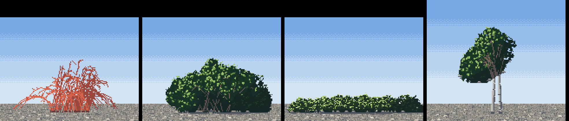
148. First try: winter willow, Sitka alder, dwarf willow, red alder.
Bare tree crowns needed their own painter. The wand fan made brooms and feather dusters, however I set it (151–153). A recursive fork does it: 5–7 main branches, each forking 2–3 ways, shorter and more spread each time, clipped to an oval, the last generation a haze of single twig pixels. Then it was too much haze, a mauve cloud (164), until only the second generation emits sparse twigs.
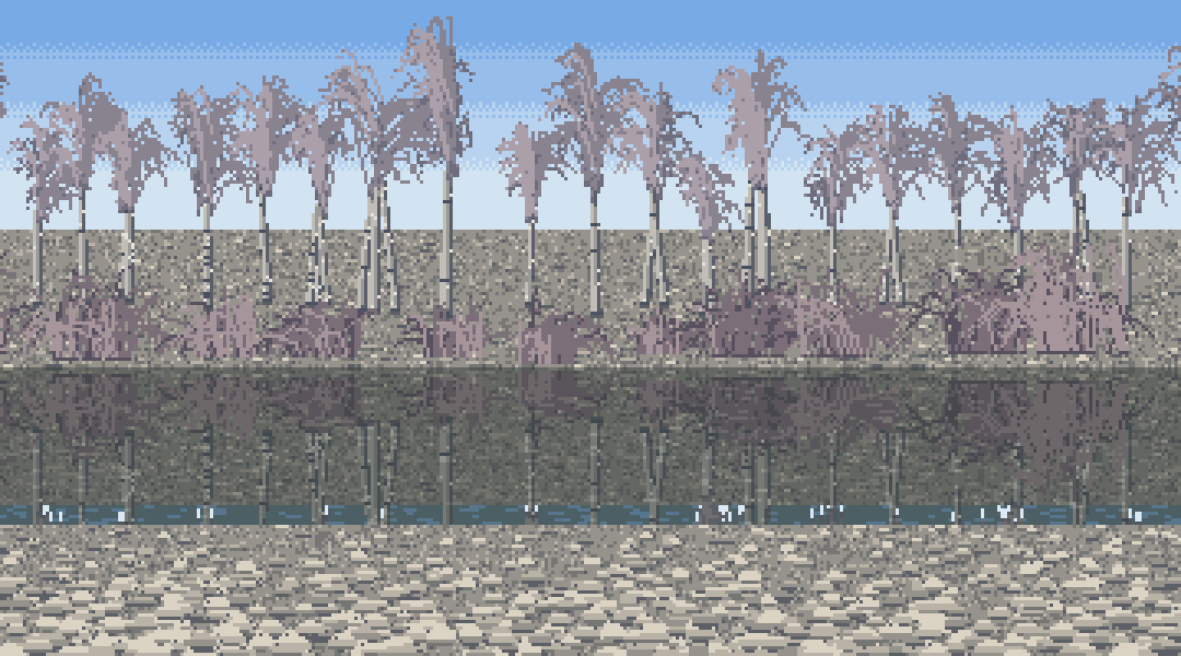
153. Bare alders from the wand fan: feather dusters.
Two trunk bugs. In the first cottonwoods a pale band crossed every trunk (157). Two causes. First, limbs painted after the trunk overwrote it at the junction with their own lit side; now the first painter of a pixel keeps it. Second, the trunk rasteriser sampled one point per pixel of segment length, and on a leaning segment two samples sometimes rounded onto the same row and skipped the next: a whole missing row that showed the sky. I found that one by printing materials down a trunk column and seeing a row of 1 (sky) inside a column of 14 (bark). Oversampling 2× fixed it.
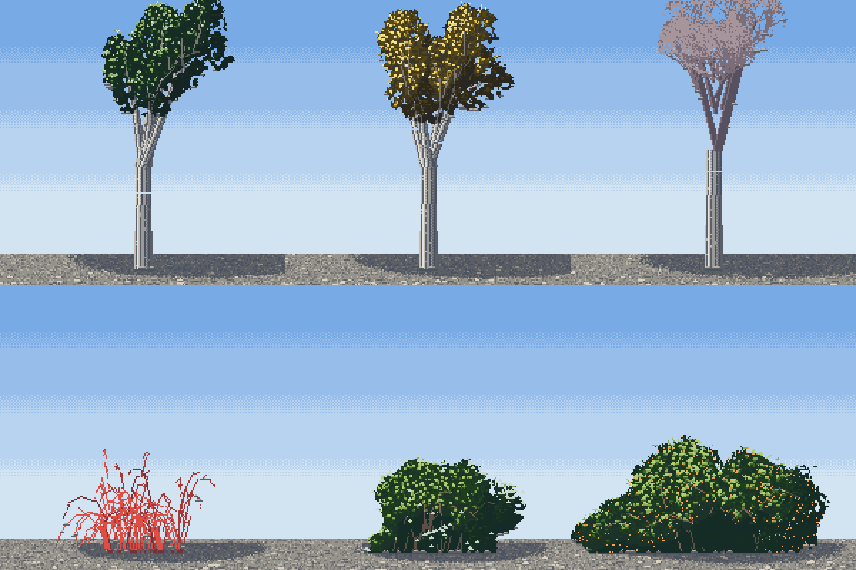
157. The first cottonwoods. See the pale line across each trunk.
Per-species palettes. In the first autumn riparian scene, one palette per scene turned the alders gold (160). Alders drop their leaves green-brown. Materials went 16-bit (group offsets past 255 would have wrapped in 8 bits) and each species group got its own seasonal palette.
Groves. The coordinator pointed out that my alder trunks stood at even spacing, "a colonnade", a failure the second critic had flagged across the studio. Stand positions now come in clusters of 1–5 with uneven gaps, trunks leaning at random.
One last bug is worth telling because it nearly got past me. A bush placed mostly off the canvas edge left a foot too narrow to sample, and rng.uniform(low, high) threw on high < low. The whole scene run died, and the old images stayed on disk. I noticed only because the "new" winter render looked identical to the last one. Check timestamps; a render that didn't change probably didn't run.
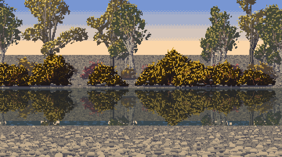
173. The riparian stand in October: ragged yellow cottonwoods above green-brown alders, gold willow on the bar, purple-red dogwood at the bank toe.
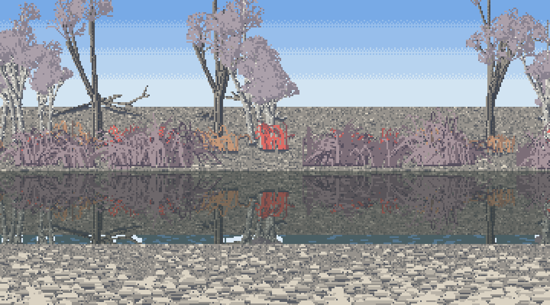
The same river in winter: bare alders as lace over white trunks, red dogwood and orange salmonberry canes along the bank.
What I'd tell someone starting
- Copy first, from the indices, until you can say what the master is doing in one sentence. My physics bush was an hour of lighting without an idea. The copy gave me the idea (clumps are a light field; marks are drawn from it), and every later stage is that idea plus an observation.
- Metrics are instruments, never judges. My best blur score was my least structured copy; the search matched every statistic and missed the clumps.
- Look at a photo before you change anything. Hanging leaves, drooping skirts, the back-lit glow and the see-through base all came from photos, each one after I'd tried to invent the answer.
- Every failure has a name, and the critic was usually right about it. Sponge, haystack, teddy bear, lace, cracks, ledge, stickers, puddle, Rorschach blot, colonnade. Each name pointed at one missing rule.
- Check that a render actually ran.
The honest state of the work: at 60–150 px in colour it reads as willow scrub. The copies never reached Ferrari's bar at 8×. A lone cottonwood reads as one only on good seeds, the dwarf willow is a hedge rather than a mat over rock, and my gravel still lies in rows (the channel and cobbles students have better gravel). The things other people judged ready were the narrow hanging leaf with its silver undersides, contact with grass overlapping the foot, cast shadows made of the ground two steps darker, and the one-canvas, many-palettes season × hour system. Those are what I teach in the tutorial.