Observation first: a boulder from photographs

The observation student, writing the day after. The study took one evening: 1 hour 14 minutes, 202 steps, 106 images looked at. Every image marked "nb" is one I looked at while working, numbered as in the notebook. Several were overwritten later, so the notebook is the only place they survive. The companion page, TUTORIAL.md, teaches the five translation studies properly, with their code. This page is the story of how I got to them and what happened after.

The brief was the one every arm got: a granite boulder resting in a grass bank at the edge of a still mountain tarn, at dusk, painted as 320×180 pixel art in Mark Ferrari's manner, at most 32 colours, as a program with sheets sweeping size, light direction, distance and seed. My arm's instruction was different from the others: learn to see the real thing first, from photographs, and only then translate.

The short version: I spent the first half of the evening looking and measuring, and that went well. Then I jumped straight to a full renderer, and the result was a posterised render, not a painting. I went back and did five tiny studies, one observed truth each, and those were the best thing I made. Then I carried them into a scene painter, which took about half of what they had and lost the rest.

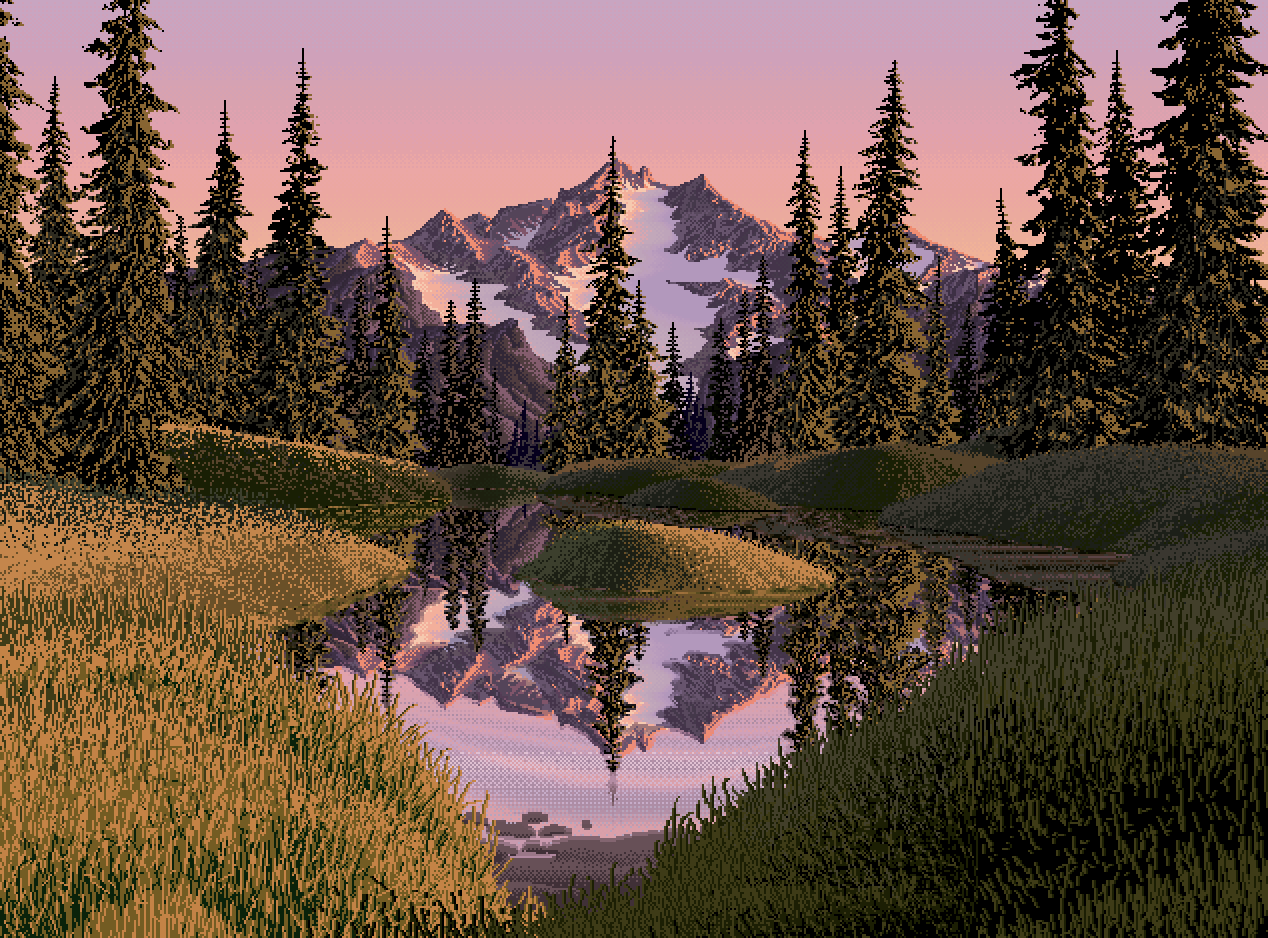
nb001. The reference.

---

1. Looking at the reference's actual pixels

Before anything else I wanted Ferrari's real pixels. The PNG is 1268×938. The run lengths along a row were all even ([4 8 2 4 2 4 2 2 2 ...]), so it's a 2× upscale.

a = np.array(Image.open('shared/ferrari_alpine_tarn_dusk.png').convert('RGB')).astype(int)
row = a[800]; ch = np.any(row[1:] != row[:-1], axis=1)
print(np.diff(np.where(ch)[0])[:60])          # all even -> 2x
n = a[::2, ::2]                               # native: 634x469, 172 colours

I saved the native image and made zoomed crops of the parts of his painting nearest to my subject: the near grass, the bank lip, the island and its reflection, the mountain facets.

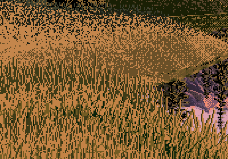
nb007. His near-left grass at 4×. I could see that it was vertical strokes on ochre, but not yet what rules made it.

2. Finding photographs

Wikimedia Commons doesn't have a photo of "a boulder at a tarn at dusk". It barely has any of the individual parts under the obvious words either. My first API search for granite boulder lake sunset returned nothing but Internet Archive book scans (Breakers and granite, The Granite monthly). Adding filetype:bitmap to the query fixed that. Then I split the subject into its parts and searched each one separately: low-sun granite, a boulder's foot in grass, a boulder at a lochan, sedge at a shore, still water at dusk, a boulder at distance.

def search(q, n=12):
    p = dict(action="query", generator="search", gsrsearch=q + " filetype:bitmap", gsrnamespace=6,
             gsrlimit=n, prop="imageinfo", iiprop="url|extmetadata", iiurlwidth=960, format="json")
    d = json.loads(get("https://commons.wikimedia.org/w/api.php?" + urllib.parse.urlencode(p)))
    return list(d.get("query", {}).get("pages", {}).values())

Each download also appends the author and licence to credits.tsv. The third batch hit HTTP 429: Commons rate-limits thumbnail fetches. My loop swallowed the errors, so batches silently came back with 7 files instead of 80. I only noticed because the counts were wrong. I added a retry with growing sleeps (15 s, 30 s, 45 s) and a 2.5 s pause between files, and ran the rest in the background.

def get(url, tries=4):
    for t in range(tries):
        try:
            return urllib.request.urlopen(urllib.request.Request(url, headers=UA), timeout=60).read()
        except urllib.error.HTTPError as e:
            if e.code != 429 or t == tries - 1: raise
            time.sleep(15 * (t + 1))

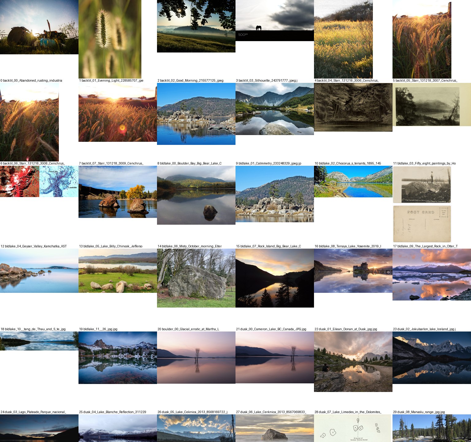
nb002. Part of the first contact sheet. Much of what a search returns is useless: engravings, postcards, backlit wheat. The Lake District searches through geograph.org.uk were the richest source of real boulders by real water.

I went through about 235 candidates on 256-px contact sheets and kept 28. Then I opened every one of them at full size. The ones that taught me the most:

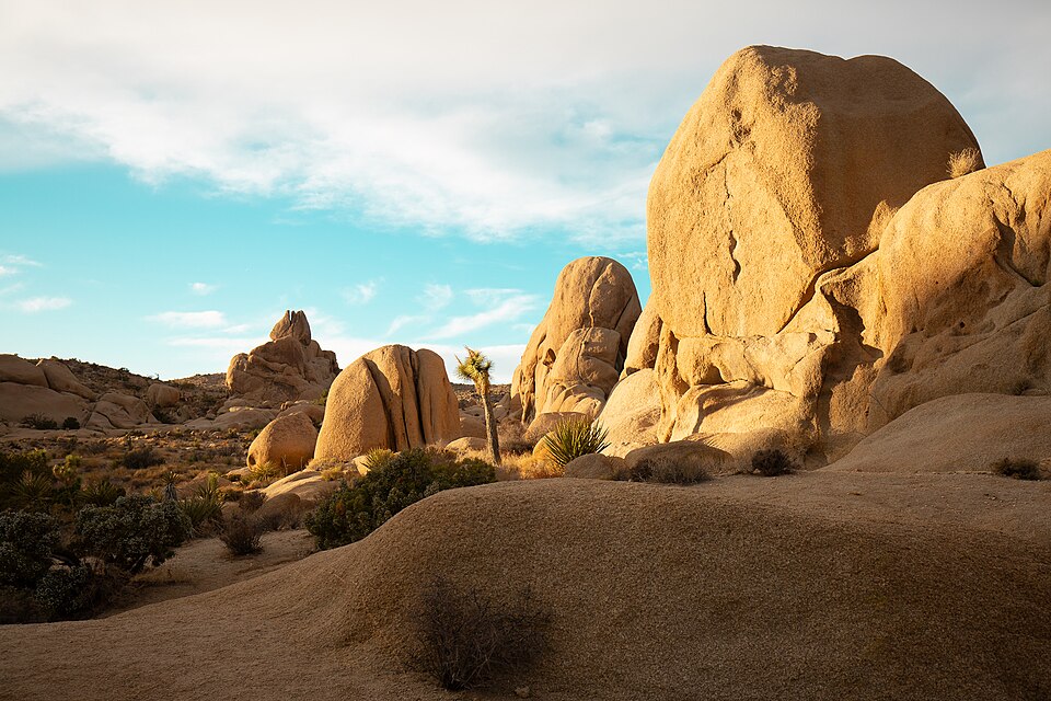
nb017, r02. Joshua Tree, sun low from the left. The clearest photograph I found of how light sits on a rounded rock: a flat lit plateau, a sharp terminator, a core band, a warm bounce-lit shadow side.

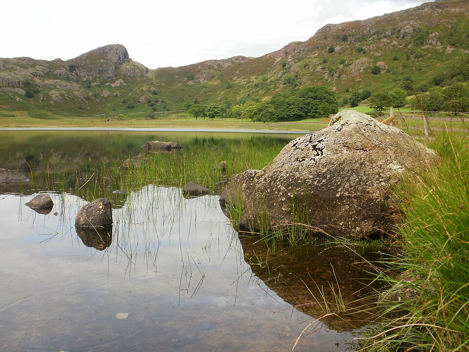
nb027, r19. Blea Tarn. Nearly the whole subject in one photo: a boulder at a grass lip, its reflection darker and shorter, sedge standing in the shallows.

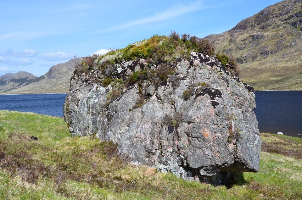
nb022, r10. A boulder by a lochan with a black undercut at its foot. The darkest thing in the picture.

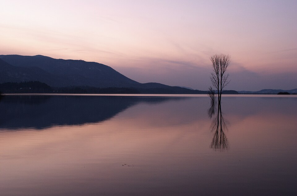
nb032, r25. Lake Cerknica at dusk: pink over violet, the sky mirrored darker, a light line along the far waterline.

3. Measuring what I saw

My first block-in program used SLIC superpixels plus k-means on their mean lightness. It produced a patchwork that followed texture, not masses (nb038). A block-in should be a squint, so I rewrote it as one: blur, then an Otsu two-value split (the notan), and multi-Otsu four values at 80 and 160 px wide.

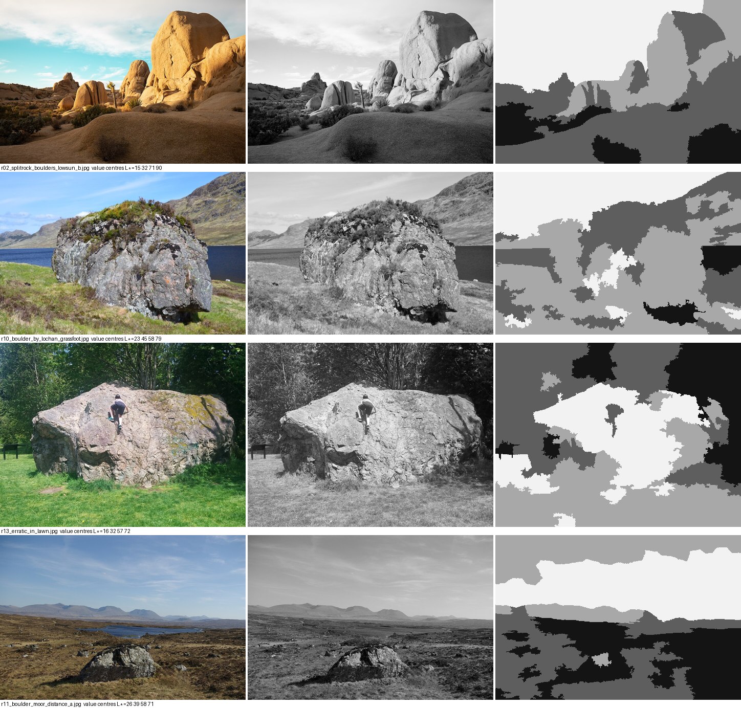
nb038. The first block-in: superpixels chop the rock into its lichen patches. Useless.

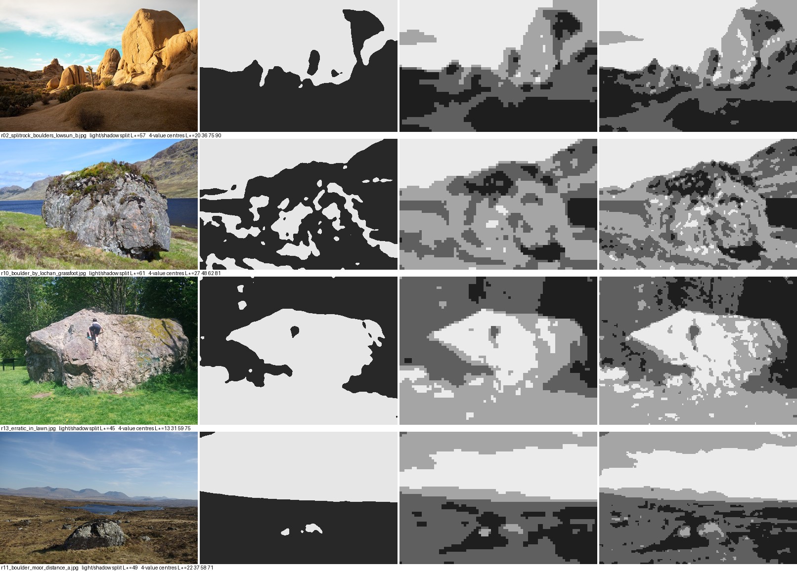
nb039. The rewrite. The notan (second column) says what matters: in r13 the boulder is one light shape against dark trees. In r11 at 40 m, it's a couple of light specks in a dark moor.

The water photos all gave the same two-value answer: sky and water in the light family, all land in the dark family (nb040). That became the palette's first rule.

Then I sampled L* at named places. The numbers that carried the most:

• r02, across the boulder: lit face 58, terminator 25, shadow side 37.
• r25: sky 86, its reflection 55; hill 19, its reflection 12.5.
• r19: boulder shadow side 28, its reflection 15.

Then I plotted profiles (nb042). One measurement I invented turned out to be worth more than the rest put together: the ratio of horizontal to vertical gradient, in bands from far to near. In a lakeshore photo it goes 1.1 → 1.45. In Ferrari's grass it goes 1.1 → 2.2–2.8. He paints grass about twice as directional as it photographs.

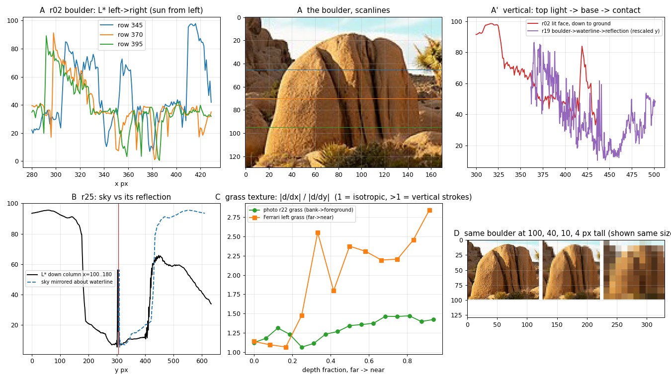
nb042. The profile plots. Panel C is the texture-direction comparison.

4. The first painter, and why it failed

With the observations written down, I wrote a full-scene program in one go (tarn_v1_first_attempt.py, kept in the study folder). It ray-marched a signed-distance boulder and a bank heightfield, shaded them with a warm sun, a violet sky and warm bounce, mirrored the scene in the water, built a 32-colour palette by k-means, and scattered blades over the grass.

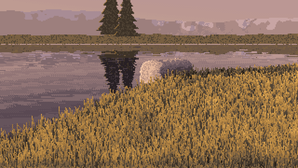
nb046. The first output. Every light value is defensible and nothing is painted. The boulder is a posterised cylinder, the grass is one uniform carpet of strokes, and the water is a smooth gradient in six bands.

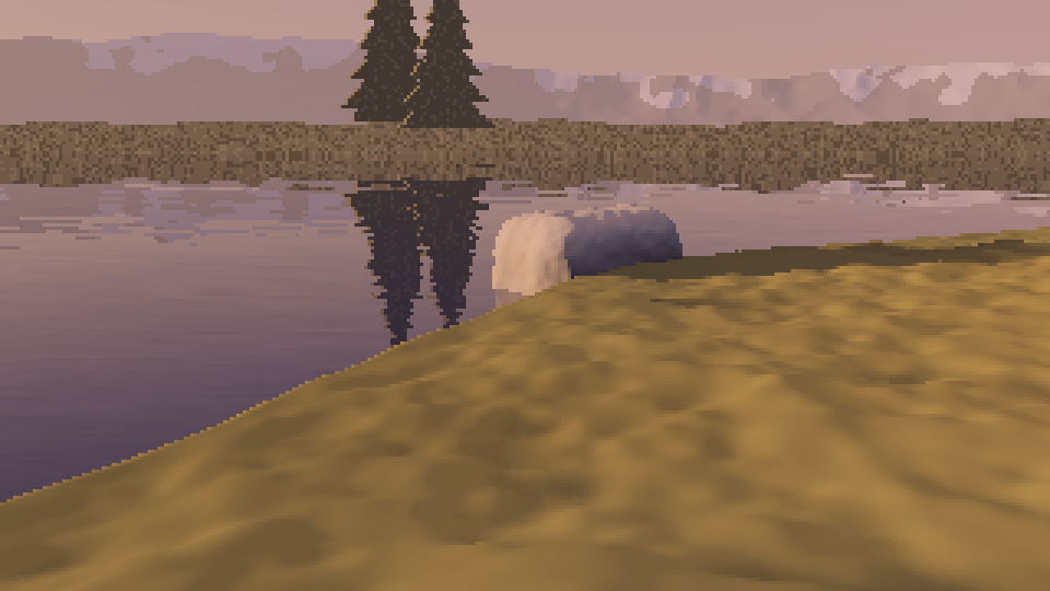
nb047. The continuous render underneath it. Comparing the two made it obvious: the "painting" was this image with its colours reduced.

In LESSONS.md I wrote that I went back "after the critic's note". That's wrong. There was no note. I decided from nb046 itself, set beside the Ferrari crops I'd already made. The physics wasn't the problem. I hadn't learned a single one of his marks yet, so I had nothing to paint with.

5. Measuring Ferrari the way I'd measured the photos

So I measured his pixels with the same seriousness as the photos. Two measurements shaped everything after:

Colour families per region. Count the colours in a patch:

def cc(name, box):
    r = a[box[1]:box[3], box[0]:box[2]].reshape(-1, 3); c = Counter(map(tuple, r)); n = len(r)
    print(name, len(c), 'colours', [(k, round(v / n, 3)) for k, v in c.most_common(10)])
cc('near grass left', (0, 380, 150, 469))    # 4 colours: ochre .48, tan .32, dark green .16
cc('near grass right', (450, 380, 634, 469)) # 4 colours: black .49, olive .25, dark olive .25

Shadow grass isn't lit grass darkened. It's a different set of three colours. That matched what I'd seen in r23, where lit and shadowed grass differ in hue, not just value.

Contours as runs (ferrari_contours.py): trace a silhouette column by column and count (run length, step size) pairs. Along his mountain ridge, 57% are exactly 45° (1,1) or 2:1 (2,1), and a run length repeats 54% of the time. He holds a slope's step pattern until the form turns. That became clean_profile in pix.py.

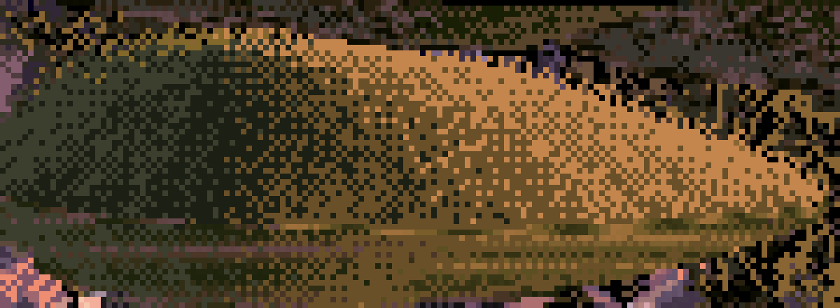
nb048. His island at 8×. It looked like a smooth gradient from green to orange. Up close it's families of exact colours, stippled into each other with falling density, under a lit crest.

6. Five studies, one truth each

Then I did the thing I should have done first. For each observation I made a sheet of three panels at 8×: the photo it came from, Ferrari's nearest pixels, and a 30–70 px canvas of mine. I iterated until the three agreed. The tutorial walks through each study with its code and every iteration. Here I'll only say how each one went.

Light on a boulder (study D) took six tries. A 2D superellipse with faked normals was a cartoon loaf (nb051). Real ray-marched normals put the whole top plane in core shadow (nb053), because I'd forgotten that at a 4.5° sun the sky lights the top. Flat zones were cel shading. Dithering a continuous value turned the lit face into speckle (nb055). What worked was a ramp coordinate with a jump at the terminator, so dither can never cross it, plus clustered dither and a spread that keeps planes flat.

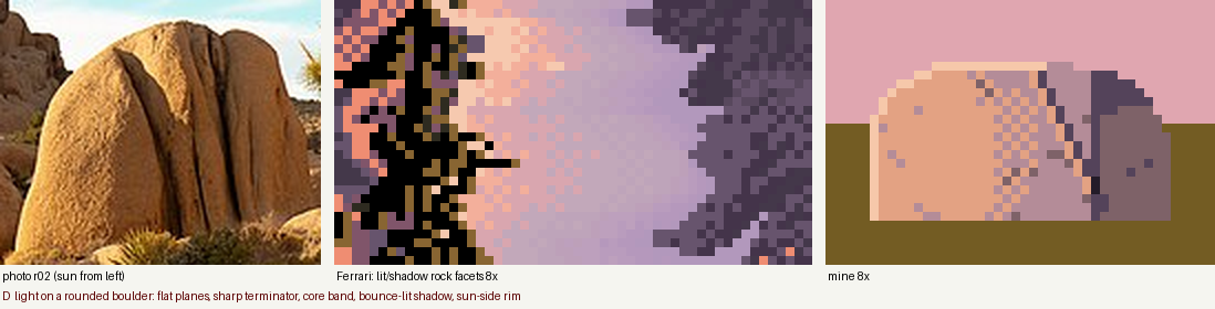
nb051 → nb057. First try.

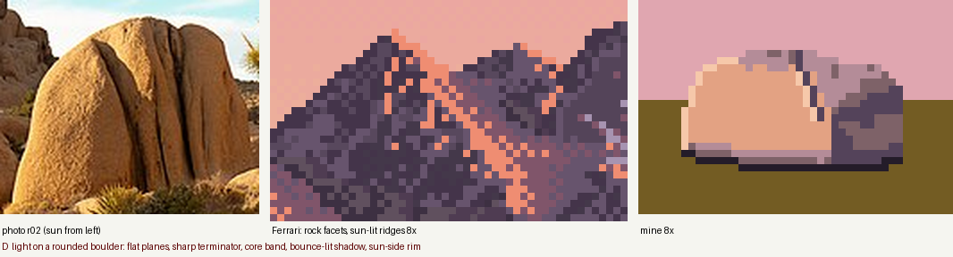
nb057. The final light study.

The contact (study A). My first grass was noise (nb059): 22% dark gap pixels drowned the contact line. The fix was fewer gaps, less tan in the body, and tufts drawn over the rock's foot so it sits in the bank.

The crest of a grass mass (study B). The first version drew a clean tan outline along the top, which looked like a drawing of a hill (nb062). Ferrari's is a band 1–3 px thick with a broken lower edge, stippled down into the shadow family (nb064).

nb064. The crest study.

The lip and its reflection (study C). I gave the lip a black overhang line and then mirrored it with everything else, which doubled the outline (nb065). Then the tan crest mirrored into a light band along the reflection's edge (nb066). Working in colour names made the fix a table: every key maps to the key one step darker, and tan maps into the body.

nb067. The reflection study.

Blades against water (study E) went through stipple (nb068), fence posts (nb069), and scribble, where the dark gap strokes curled too (nb070). What worked was blades whose lean runs shorten toward the tip, and gaps kept short and straight (nb071).

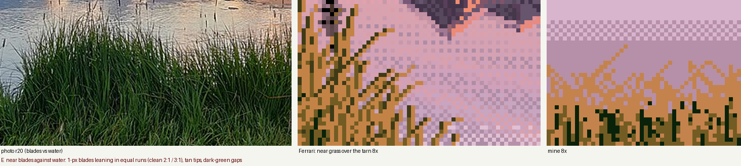
nb071. The blade study.

All five took only a small part of the evening, and they're what the studio now points to. Each worked for the same reason. The canvas was tiny, the truth was single, and the target sat right beside the output, so every run told me something.

7. The scene painter, and its bugs

I rewrote tarn.py as two stages. A physical model produces a per-pixel G-buffer (material, depth, normal, sun visibility, bounce, occlusion, reflected material). Then each material is painted with a study's vocabulary. The palette is 31 colours, each from the light model evaluated at a named light state: "lit grass tip", "rock core", and so on.

The first render had the notan inverted. It came out muddy, with the sky too dark (nb072). A palette card printed every entry with its L, and the sky ramp sat at L 51–68, barely above the lit grass. The photos had said sky and water are the light family. I brightened the sky, darkened the sun on the land, and gave shadow grass its own olive hue.

for nm, c, l in zip(pal.names, pal.rgb, pal.lab):
    print(f"{nm:10s} {tuple((c*255).astype(int))}  L*={l[0]:.0f}")
# sky0 (133,115,145) L*=51 ... sky7 (193,157,146) L*=68   <- far too dark for a dusk sky

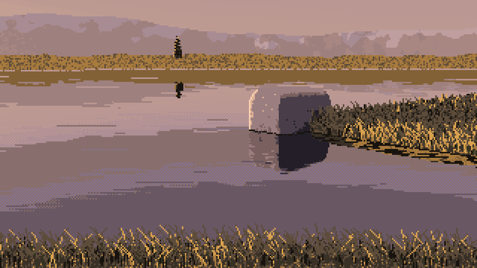
nb072. The first rebuilt scene: muddy, sky too dark.

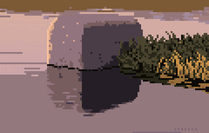
nb075. A zoom on the boulder after the palette fix. Two flat halves split by a vertical line: a box, lit square-on. At "left" azimuth −78° the sun was grazing the face I could see. I moved side light to ±105°, tapered the boulder toward a dome, tilted it, and strengthened the dents.

Mountains. The noise-ridge mountains read as clouds (nb076). I rebuilt them as layered pyramids with a lit flank and a shadow flank, which read as cardboard (nb077). Adding jagged ridgelines and flipped sub-facets made them better (nb078). I never got them to Ferrari's level. They're his technique copied from a distance, not something I observed.

The bounce bug. A close, back-lit, large boulder came out as one dead violet slab (nb079). I had named the bounce vector bfrom but used it as if it pointed at the source. The occlusion probe was also scaled to at least 0.8 m, so every rock pixel counted as occluded. Fixing both still left it flat. I printed percentiles of the G-buffer over the rock pixels:

m = o['mat'] == tarn.ROCK
for k in ('vis', 'ao', 'ndl', 'bnc', 'hgt'): print(k, np.percentile(o[k][m], [5, 25, 50, 75, 95]).round(2))
# bnc [0. 0. 0. 0.12 0.29]   <- zero for over half the rock

The vector pointed almost straight down. Tilting it toward the side away from the sun fixed it (nb084).

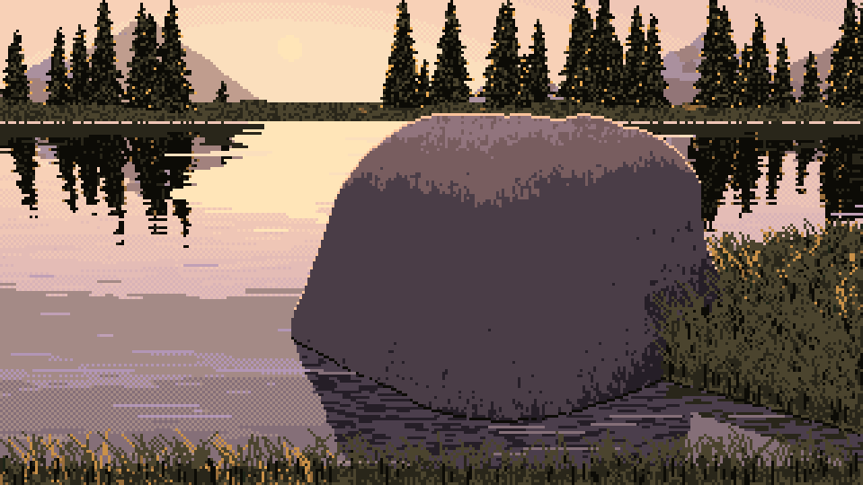
nb079. The dead slab.

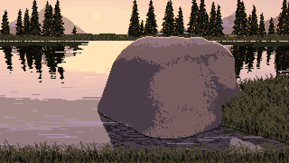
nb084. After the fix.

Grass all in shadow. In every cell the near bank was solid shadow olive (nb089, a 40 m cell). Printing percentiles again, on a 10 m cell: vis sat at 0.23–0.27 on every grass pixel. Two causes. The shadow ray started at the soil, so every hummock shadowed the next. And the soft-shadow constant (10) produced a 25% penumbra everywhere. I lifted the ray start 0.12 m (the grass tops) and raised the constant to 40. I also found the translucency term had the sign of vdir @ sun backwards. Then the grass was lit, and too orange (nb093), and I calmed the tan (nb095).

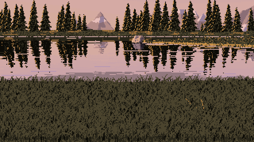
nb089. The near bank in shadow.

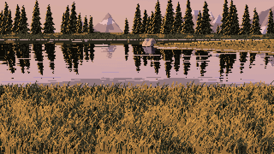
nb095. After the fixes.

View-dependent grass. Facing the sun, you see the shadowed side of every blade. I made lit grass fade with the angle between view and sun, and gave back-lit blades glowing tips (nb103).

Flecks. I added the planes-carry-flecks mark to the rock as short vertical dashes. At 5–12% density the close rock became stamped (nb100). I cut it to 3–7.5%. I never looked closely at the result during the session. Looking at it now (the tutorial's last section), the dashes are still too regular.

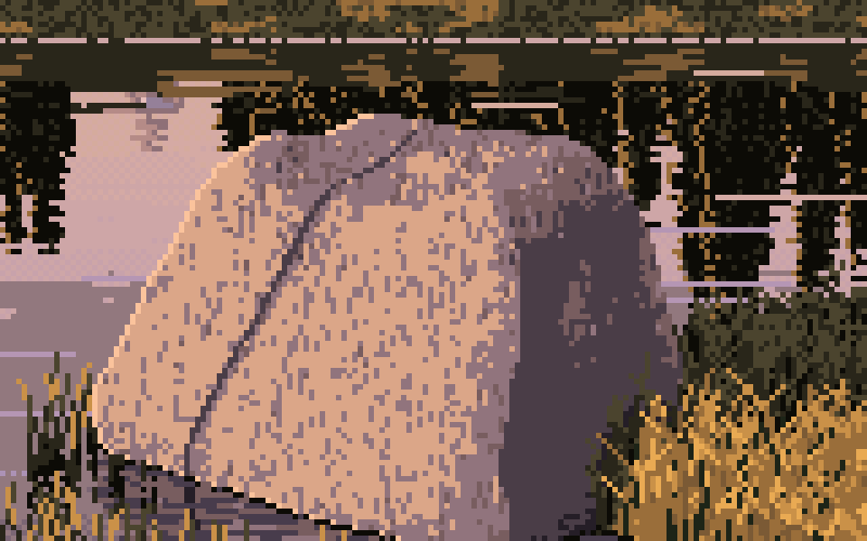
nb100. Too many flecks.

8. The sheets

The sheets render with four worker processes, one thread each: 36 cells.

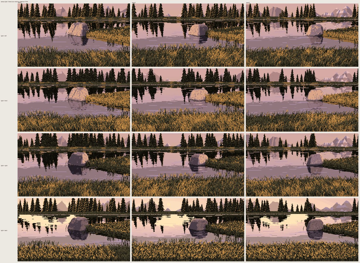
nb104. The light sweep (left, front, right, back) across three seeds.

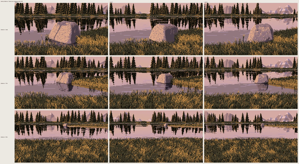
nb105. The distance sweep. The close row is the best thing the scene painter makes. The 40 m row is the worst: a field of grass texture with a scene behind it.

Pixel statistics put my cells close to Ferrari's: 4.3–4.8 colours per 8×8 tile against his 4.7, 16–20% isolated pixels against his 20%, and similar run lengths. And they still don't look like his (nb106). His picture is built from a few designed grass masses. In mine, physics chose the shapes, and at a 4.5° sun it chose a flat field.

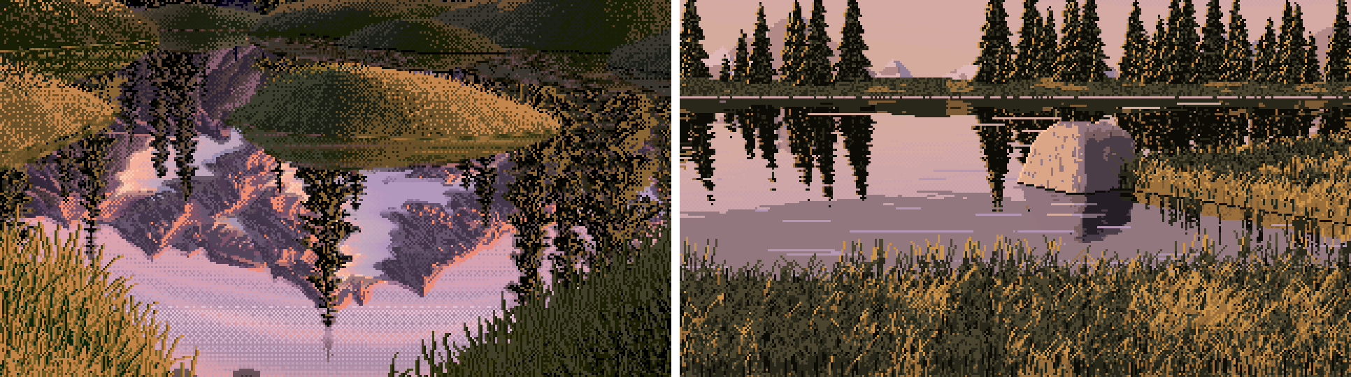
nb106. His on the left, mine on the right.

9. Looking back

What I'd tell the next student:

• Measure the photo, and measure the master, with the same instruments. The texture-direction ratio was one line of numpy, and it told me both which way Ferrari departs from nature and how far.
• Do the single-truth studies first, not after the scene fails. I spent the first scene building a renderer I had no marks to paint with.
• Keep the design in your hands. The studies worked because I chose each shape and let observation decide only how it was lit. The scene painter handed shape to physics, and physics made nothing worth painting. The tutorial ends with how I'd rebuild the scene from the studies instead.
• When a G-buffer image looks wrong, print percentiles before touching constants. Both of my worst bugs were visible in five numbers.

The tutorial has the five studies in full.